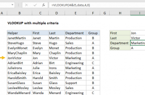
All data is in an Excel Table nameddatain the range B5:E14.
This means the formulas below usestructured references.
As a result, the formulas will automatically include new data added to the table.

Because we want OR logic, we use addition in this case.
Notice Excel is not case-sensitive, so we don’t need to capitalize the colors.
In the second array, TRUE values correspond to “pink”.

This means the values are mutually exclusive both tests can’t return TRUE at the same time.
This creates a new array containing only TRUE and FALSE values.
Video:Boolean algebra in Excel.
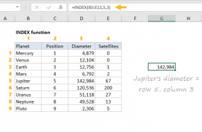
Thecolumn_numargument is hardcoded as 0 to tell theINDEX functionto return theentire row.
Because this formula returns 4 values in one row, it must be entered as amulti-cell array formulainLegacy Excel.
InExcel 365and Excel 2022, the formula “just works” and all four valuesspillinto multiple cells.

For more on this behavior, see:Dynamic Array Formulas in Excel.
XLOOKUP supports approximate and exact matching, wildcards (* ?)
it’s possible for you to use INDEX to retrieve individual values, or entire rows and columns.

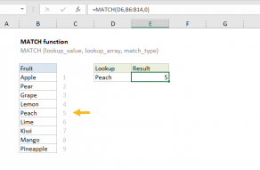
MATCH supports approximate and exact matching, andwildcards(* ?)
Often, MATCH is combined with the…
Related videos
Boolean algebra in Excel