The beauty of TRIMRANGE is that it will track the data in a worksheet as it changes.
See below for details with examples.
This article is focused on TRIMRANGE, but includes a section on Trim Refsbelow.

The result is a “trimmed range” that includes only the data in the original range.
Essentially, trim refs use a dot (.)
together with the colon (:) in a range to add trim behaviors.
Personally, I prefer the TRIMRANGE function because it makes the action clear and explicit.
The dot syntax is tricky to read and might not be noticed or understood by many users.
How TRIMRANGE works
It’s important to understand how TRIMRANGE works.
Starting from the outer boundary of the range, TRIMRANGE scans inward.
It removes empty leading and trailing rows, and empty leading and trailing columns.
The final result is data in the range B3:H14.
What is a dynamic range?
To understand why TRIMRANGE can be useful, you should understand the concept of a dynamic range.
A dynamic range in Excel automatically expands and contracts to track the data it contains.
The beauty of this approach is simplicity.
Instead of working out the address of the last row that contains data, we just provide columns.
However, we must be careful because Excel worksheets are very large each worksheet contains over 1 million rows.

Essentially, TRIMRANGE allows us to have our cake and eat it too.
We can use simple references and let TRIMRANGE figure out which cells contain data.
More commonly, you will pipe the result of TRIMRANGE into another function.

By default, TRIMRANGE trims empty rowsand columnsfrom a range.
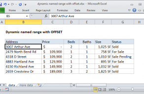
The table that holds the property listings appears in the range B4:H14.
The first row is a header row, so the actual data range is B5:H14.

This doesn’t quite work in this case because we are including the header row together with the data.
We can solve that problem by adding the DROP function to drop the first row.
The next logical step is to create a dynamicnamedrange.

One way to do that is to create anamed range.
A named range is simply a human-readable name assigned to a range.
Because formulas respond to changes in a worksheet, we call this a “dynamic named range”.
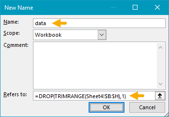
The first step is to define a name.
This is because we need to the reference to work the same from any cell in the workbook.
First, we have reduced redundant code in our formulas.

As before, the range is fully dynamic and will adapt as the worksheet is changed.
Because we are using TRIMRANGE, these formulas are dynamic and will instantly update when products or colors change.
Note we are not using TRIMRANGE to create a dynamic named range in this case but we could.

For more details on Data Validation, seethis page.
Example - Anchoring other formulas
Another use of TRIMRANGE is to “anchor” other formulas.
What does this mean, exactly?

This is convenient because we get all 1 results with a single formula.
With TRIMRANGE, naturally .
In the worksheet below, we have the original formula in cell D5.

However, remember that TRIMRANGE trims the rangefirst, before DROP gets involved.
There are different ways to handle this kind of problem.
Key benefits of TRIMRANGE
TRIMRANGE is a technical function designed for more advanced users.

The number of rows and columns to remove is provided by separaterowsandcolumnsarguments.
By default, TOCOL will scan values by row, but TOCOL can also scan values by column.
TOROW Function
The Excel TOROW function transforms an array into a single row.

By default, TOROW will scan values by row, but TOROW can also scan values by column.