Explanation
This example shows a workbook designed to apply discounts based on seven pricing tiers.
The total quantity of items is entered as a variable in cell C4.
The discount is applied via the unit costs in E7:E13, which decrease as the quantity increases.
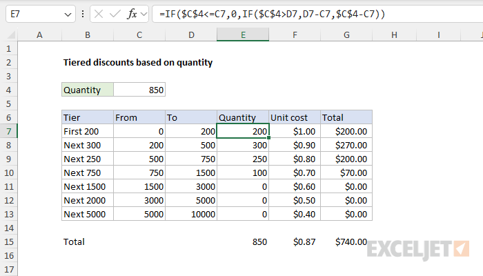
The first 200 items have an undiscounted price of $1.00.
The next 300 items have a discounted unit price of $0.90.
The next 250 items have a unit price of $0.80, and so on.
The main challenge in this problem is calculating the correct quantities in the range D7:D13.
We fill one bucket at a time, beginning with the first tier.
Once that bucket is full, we move on to the next bucket.
The first method keeps the worksheet structure intact and uses the MAP function to generate all tier quantities simultaneously.
This method requires Excel 365.
Then, we use the DROP function to remove the final last value since we don’t need it.
Next, we have a customLAMBDA calculation.
(See ourMAP pagefor an explanation of this structure).
However, it is also a case where choosing MAP is not obvious.
Knowing when and how to do this is part of the learning curve of new functions like MAP.
I’m sure there are many ways to solve this problem with other dynamic array functions.
This approach processes each row individually.

VSTACK Function
The Excel VSTACK function combines arrays vertically into a single array.
The number of rows and columns to remove is provided by separaterowsandcolumnsarguments.
More than one condition can be tested by nesting IF functions.

The MIN function ignores empty cells, the logical values TRUE and FALSE, and text values.
MAX Function
The Excel MAX function returns the largest numeric value in the data provided.
MAX ignores empty cells, the logical values TRUE and FALSE, and text values.