The problem is that the formula area in a conditional formatting rule isn’t very friendly.
Luckily, there’s an easy fix:dummy formulas.
This may at first seem impossible how can you test a conditional formatting formula without applying a conditional format?
When a formula in the overlay returns TRUE for a given cell, the formatting is applied.
This makes it easy to set up and match references.
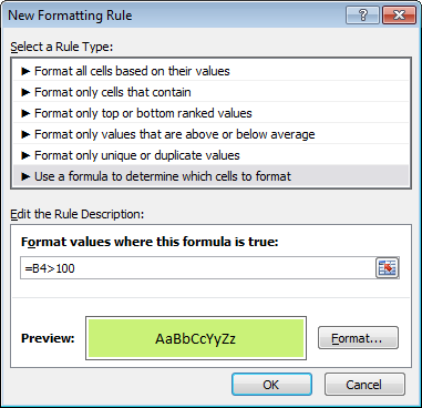
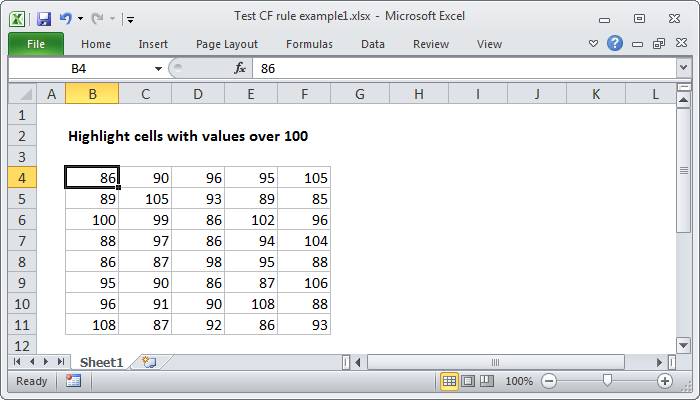
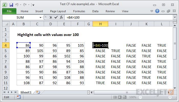
Then, simply write the first formula by referencing the upper left cell in the data.
This will be the active cell when the conditional formatting rule is created.
We are just using a basic formula as an example.
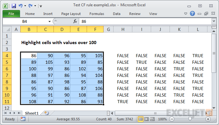
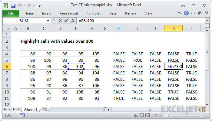
We have plenty of space to the right, so we’ll add our dummy formulas there.
In cell H4, add the first formula.
In this case, we want to use:
Why B4?
Because B4 corresponds to the active cell we’ll have when we define the actual conditional formatting rule.
Now copy the formula across and down.
You only need to copy down as many rows as you want to test.
In this case, with a small set of data, we can easily test all rows.
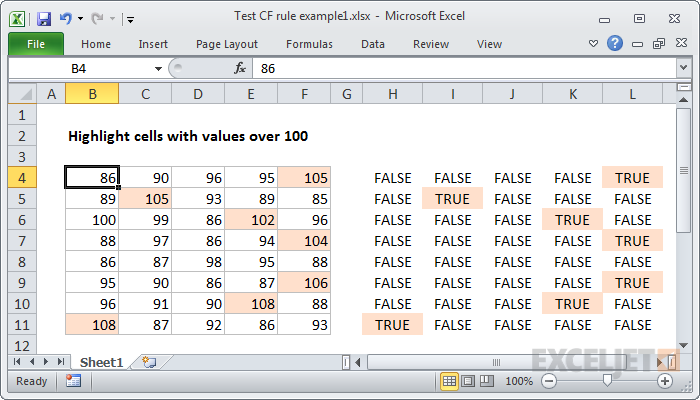
Notice we get a TRUE or FALSE value in every cell.
All references to B4 have changed, since B4 was entered as a relative address.
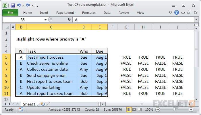
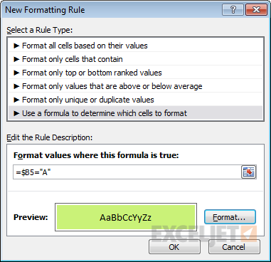
Next, choose the data and define a new conditional formatting rule.

Ready to save the new rule
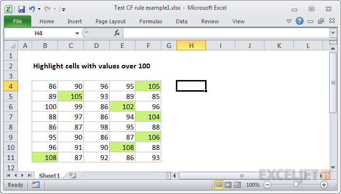
Success!
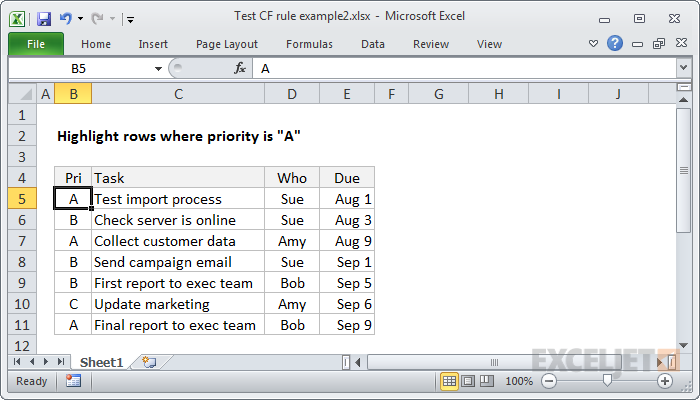
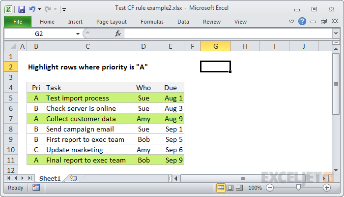
Let’s create a rule that highlights rows in a table based on the value in one column.
In this case, we’ll highlight tasks with a priority of “A”.
However, by using dummy formulas, we can easily test and perfect a rule.
As before, the first step is to figure out where to put the test formulas.
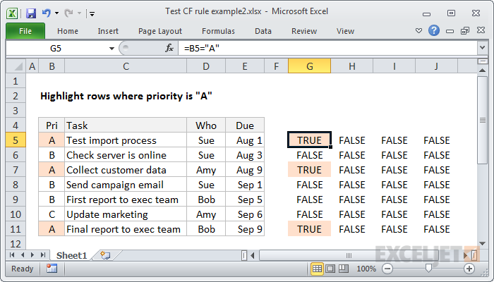
We have plenty of room to the right, so we’ll start in cell G5.
It’s a good start, but it will only highlight cells in the first column.
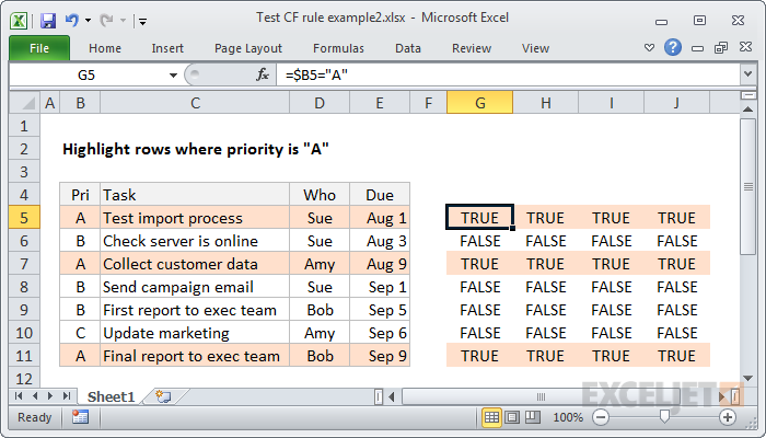
We need to adjust the formula so that it returns TRUE for the entire row.
To do this, we need to use a mixed reference in the formula to lock the column.
Imagine them as an overlay on the data itself.
Now let’s created the conditional formatting rule.