The SUMIFS function is designed to sum numeric values based on one or more criteria.
The main reasons to do this are simplicity and speed.
In the example shown, we have quarterly sales data for four regions.

The behavior of SUMIFS is to sumall matching values.
However, because there is justone matching value, the result is the same as the value itself.
Below, we look at several lookup formula options.

Lookup formula options
This section briefly reviews other formula options that yield the same result.
With VLOOKUP
Unfortunately, VLOOKUP is not a good solution to this problem.
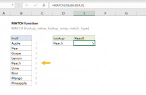
Then we can ask theMATCH functionfind the number 1.

One of LOOKUP’s key strengths is that it can handle arrays natively.
This represents the value we want to retrieve.
We use a lookup value of 2 because we can’t guarantee the array is sorted.
So, we force all non-matching rows to errors, and ask LOOKUP to find a 2.
LOOKUP ignores the errors and dutifully scans the entire array looking for 2.
The result is the same as above, 127,250.
More detailed explanation here.
With just a single array to process, the SUMPRODUCT function returns the sum of the array, 12,7250.
Seethis examplefor a more complete explanation.

In spirit, the SUMPRODUCT option is closest to the SUMIFS formula since we aresummingvalues based on multiple criteria.
As before, it works fine as long as there is only one matching result.
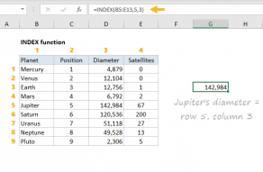
you’ve got the option to use INDEX to retrieve individual values, or entire rows and columns.

MATCH supports approximate and exact matching, andwildcards(* ?)
LOOKUP’s default behavior makes it useful for solving certain problems in Excel.
XLOOKUP supports approximate and exact matching, wildcards (* ?)


