In the latest version of Excel, the easiest way to solve this problem is with theTAKE function.
In older versions of Excel you’ve got the option to use theOFFSET function, as explained below.
TAKE function
The TAKE function returns a subset of a givenarrayorrange.

The size of the array returned is determined by separaterowsandcolumnsarguments.
Negative numbers take values from the end or bottom of the array.
For example:
In the worksheet shown,datais the named range C5:H16.

The result is a “trimmed” range that only includes the used portion of the range.
Note: theOFFSET functionis a volatile function and can cause performance problems in larger or more complicated worksheets.
If you run into this problem, see the INDEX solution below.

F5:H16).
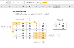
The number of rows and columns to return is provided by separaterowsandcolumnsarguments.
Rows and columns can be extracted from the start or end of the given array.

OFFSET is handy in formulas that require a dynamic range.
COLUMNS Function
The Excel COLUMNS function returns the count of columns in a given reference.
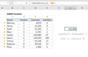
you’ve got the option to use INDEX to retrieve individual values, or entire rows and columns.
These values can be numbers, cell references, ranges, arrays, and constants, in any combination.
SUM can handle up to 255 individual arguments.
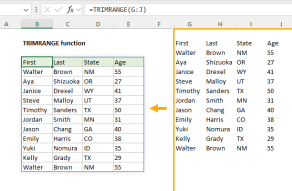
TRIMRANGE Function
The Excel TRIMRANGE function removes empty rows and columns from a range of data.

The result is a “trimmed” range that only includes data from the used portion of the range.