All data is in the range B5:B16 andnis entered into cell F5 as 3.
This value can be changed at any time.
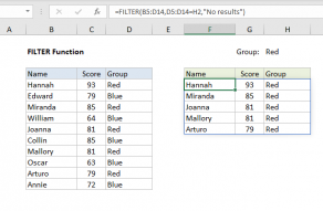
In thelatest version of Excel, the easiest way to do this is to use the FILTER function.

This is the value returned to FILTER as theincludeargument.
FILTER uses this array to “filter” values in the range B5:B16.
Only values associated with TRUE make it through the filter operation.
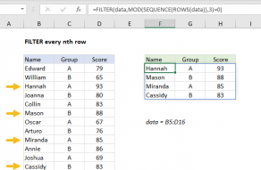
The result is an array that contains every 3rd value in the data.
Adouble negative(–) is used to convert the TRUE and FALSE values to 1s and 0s.
This formula is also dynamic.

The output from FILTER is dynamic.
If source data or criteria change, FILTER will return a new set of results.
The array can be one dimensional, or two-dimensional, determined byrowsandcolumnsarguments.
…
MOD Function
The Excel MOD function returns the remainder of two numbers after division.
For example, MOD(10,3) = 1.
The result of MOD carries the same sign as the divisor.

SUM Function
The Excel SUM function returns the sum of values supplied.
These values can be numbers, cell references, ranges, arrays, and constants, in any combination.
SUM can handle up to 255 individual arguments.

SUMPRODUCT Function
The Excel SUMPRODUCT function multipliesrangesorarraystogether and returns the sum of products.
For example, ROW(C5) returns 5, since C5 is the fifth row in the spreadsheet.
When no reference is provided, ROW returns the row number of the cell which contains the formula.

Related videos
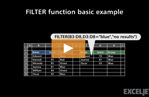
FILTER function basic example