If so, we discard the value and replace it with anempty string("").
If not, we add the non-numeric character to a “processed” array.
Change to suit your data, or use the LEN function as explained below.
This array goes into the MID function as thestart_numargument.
Fornum_chars, we use 1.
The MID function returns an array like this:
Note: extra items in the array removed for readability.

To this array, we add zero.
This is a simple trick that forces Excel to coerce text to a number.
are converted without errors, but non-numeric values will fail and throw a #VALUE error.

We use theIF functionwith theISERR functionto catch these errors.
The final array result goes into the TEXTJOIN function as thetext1argument.
Fordelimiter, we use an empty string ("") and forignore_emptywe supply TRUE.

TEXTJOIN thenconcatenatesall non-empty values in the array and returns the result.
This allows the formula to scale up to any number of characters automatically.
Removing extra space
When you strip numeric characters, you may have extra space characters left over.

With LET
We can further streamline this formula with theLET function.
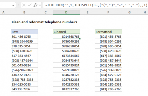
Strip non-numeric characters
you’ve got the option to use asimilar formula to remove non-numeric characters.
For example, =MID(“apple”,2,3) returns “ppl”.

ROW Function
The Excel ROW function returns the row number for a reference.
For example, ROW(C5) returns 5, since C5 is the fifth row in the spreadsheet.
When no reference is provided, ROW returns the row number of the cell which contains the formula.

INDIRECT Function
The Excel INDIRECT function returns a valid cell reference from a given text string.
INDIRECT is useful when you want to assemble a text value that can be used as a valid reference.
SEQUENCE Function
The Excel SEQUENCE function generates a list of sequential numbers in an array.

The array can be one dimensional, or two-dimensional, determined byrowsandcolumnsarguments.
…
LET Function
The Excel LET function lets you define named variables in a formula.


