The result is a dynamic summary table created with a single formula.
The result from the PIVOTBY function is similar to the output from a Pivot Table, but without formatting.
The table returned by the PIVOTBY function is fully dynamic and will immediately recalculate when source data changes.
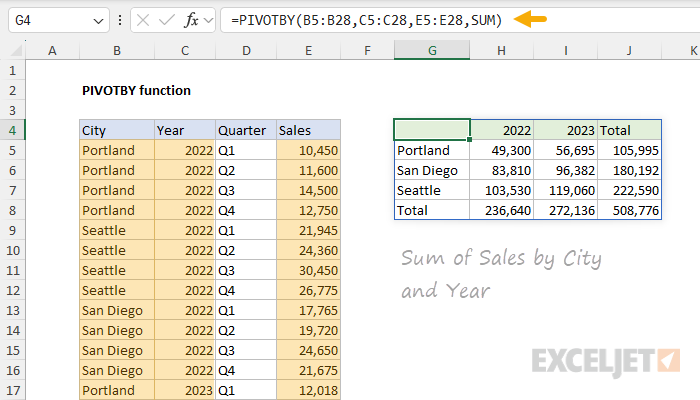
In the worksheet below, we use the PIVOTBY function to summarize sales by city and year.
The entire table in G4:J8 is returned in one step.
Notice that we have included the header row inrow_fields, col_fields,andvalues, but it is not displayed.
PIVOTBY will attempt to detect a header row automatically so that it won’t be included in value calculations.
However, PIVOTBY will not display headers in the output unless enabled explicitly by thefield_headersargument.
Note also that PIVOTBY includes a Total row and Total column by default.
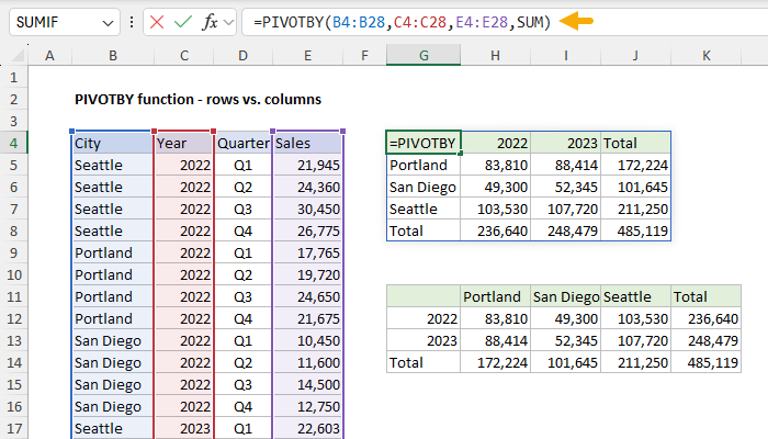
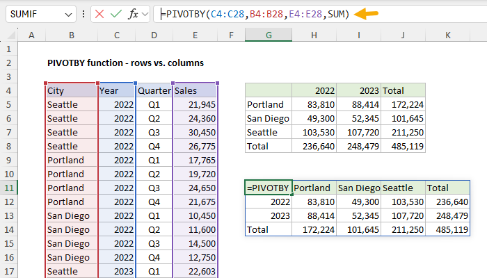
As the name suggests, the PIVOTBY function can also pivot data.
This behavior is governed by the first two arguments,row_fieldsandcol_fields.
The only difference is the orientation of the table.
The are five possible values for field_headers:
Thefield_headerargument is optional.
Whenfield_headeris omitted, PIVOTBY will have a go at detect headers in the source data automatically by testing values.
However, automatic detection only prevents the headers from being processed as values; it does not display headers.
Whencol_fieldsare included, and field headers are set to display, the resulting table can become more complicated.
In other words, you must provideeitherrow_fieldsorcol_fields, but you aren’t required to provide both.
PIVOTBY calculation options
The fourth argument in PIVOTBY is called “function”.

The function argument specifies which calculation to run when values are grouped.
you might use Excel functions like SUM, AVERAGE, COUNT, COUNTA, MAX, MIN, etc.
We use COUNTA instead of COUNT in this case because we are counting text values.
We do this because the “default” headers created by PIVOTBY in this case are not helpful.
The solution is to hardcode our own headers in G4:H4.
The formula in G4 is:
Note: the values in G4:K4 are not field headers.
They are Meal values grouped by column.
The trick is to use theHSTACK functioninside PIVOTBY to call more than one function simultaneously.
PIVOTBY automatically generates “calculation headers” when you ask for multiple calculations.

As a result, we have “COUNT” in H4 and “SUM” in I4.
To perform another calculation, we can add it to the values inside HSTACK.
Also, notice that the structure of the headers in the table is not ideal.

We’ll tackle this problem in the next section.
Depending on your use case, you may want to discard these headers and use your own.
You are free to customize these values as you like.

PIVOTBY with multiple columns
The PIVOTBY function can handle multiple columns forrow_fields, col_fields,andvaluesarguments.
When you include multiple columns, the output will have multiple row group levels.
To illustrate how this works, consider the examples below.

In the first example, we provide one column forrow_fields, and 1 column for values.
Now let’s look at what happens when we add another column (Region) torow_fields.
you’re free to also supply multiple columns forcol_fields.

When these arguments are not provided, PIVOTBY will automatically display grand totals.
If you only have a single column of data forrow_fieldsorcol_fields, you only have a depth of 1.
This means you’ve got the option to display grand totals but not subtotals.

Only by adding more columns to you increase depth and therefore make it possible to display subtotals.
In most cases, you will be working with row totals, since most reports have a vertical orientation.
As mentioned above, PIVOTBY will create and display grand totals whenrow_total_depthargument is not provided.

For subtotals to display,row_fieldsmust have at least 2 columns.
If you give a shot to enable subtotals whenrow_fieldscontains just one column, PIVOTBY will return a #VALUE!
The PIVOTBY function also supports displaying grand totals and subtotals at thetopof a group instead of at the bottom.

As the names suggest,row_sort_ordercontrols sorting for row fields, andcol_sort_ordercontrols sorting for column fields.
Both arguments are optional.
This behavior is automatic and can’t be disabled.

The number itself corresponds to the columns in the table, starting with 1 for the first column.
In other words, if the data contains 100 rows of data, thefilter_arrayshould contain 100 Boolean values.
Only rows associated with TRUE (or 1) will make it past the filter into the final output.

The Booleans in thefilter_arrayare typically generated with a logical expression.
The logical expression used forfilter_arrayisC4:C52>2023.
That’s why we can use the expressionC4:C52>2023directly to exclude years earlier than 2024.

This logic can be easily extended to include more than one condition.
In the example below, we extend the existing logical to exclude data for Seattle.
This is an example ofBoolean logic.

For a quick overview, see this 3-minute video:Boolean Algebra in Excel.
See the examples on theFILTER function pagefor examples of more complex criteria to generate a filter_array.
The PIVOTBY function does not need to use FILTER directly (because thefilter_arrayalready serves that purpose).

If you need more powerful pattern matching based on Regular Expressions, see theREGEXTEST function.
Why two syntax options?
The short form is for convenience.

It is concise and easy to read.
However, the behavior cannot be customized.
The long-form syntax uses the LAMBDA function and can be customized as needed to apply a more advanced calculation.

To illustrate this concept, suppose you want the round values that PIVOTBY returns to the nearest 1000.
The PIVOTBY function then returns the rounded sum in the final output.
A dynamic range is a range that expands and contracts as rows are added or removed.

The result is a summary table created with a single formula.
HSTACK Function
The Excel HSTACK function combines arrays horizontally into a single array.
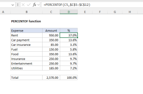
The output from PERCENTOF is a decimal number that can be formatted with Excel’s percentage number format….