Quick Links
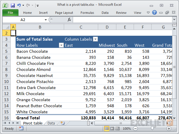
Pivot tables are a reporting engine built into Excel.
They are the single best tool in Excel for analyzing datawithout formulas.
you might create a basic pivot table in about one minute, and begin interactively exploring your data.

Below are more than 20 tips for getting the most from this flexible and powerful tool.
If you have well-structured source data, you could create a pivot table in less than a minute.
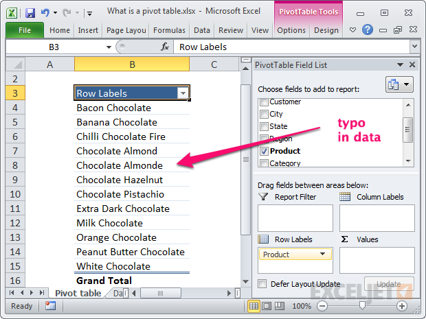
Clean your source data
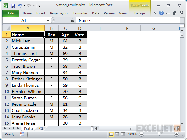
To minimize problems down the road, confirm your data is in good shape.
Source data should have no blank rows or columns, and no subtotals.
You might sometimes need to add missing data.
See this video for tips:
Video:How to quickly fill in missing data
3.
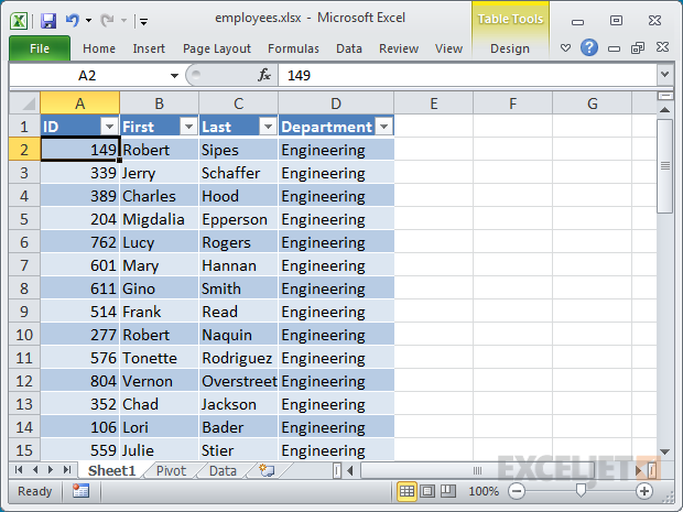
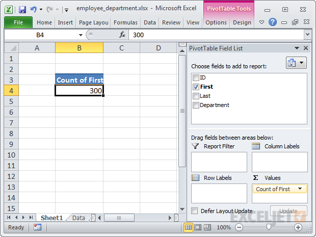
To do this, simply add anytext fieldas a Value field.
If this number makes sense to you, you’re good to go.
300 first names means we have 300 employees.
An hour later, it’s not so fun anymore.
These simple notes will help guide you through the huge number of choices you have at your disposal.
Keep things simple, and focus on the questions it’s crucial that you answer.
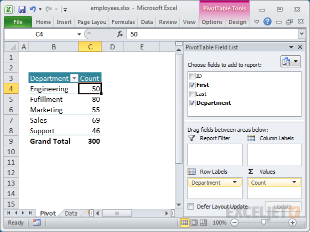
Use a pivot table to count things
By default, a Pivot Table will count any text field.
This can be a really handy feature in a lot of general business situations.
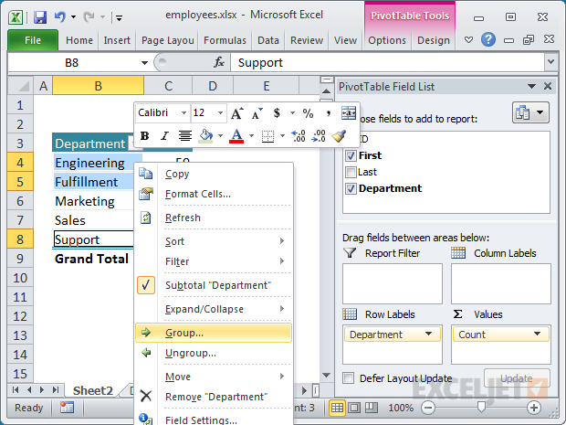
For example, suppose you have a list of employees and want to get a count by department.

To get a breakdown by department, adhere to these instructions:
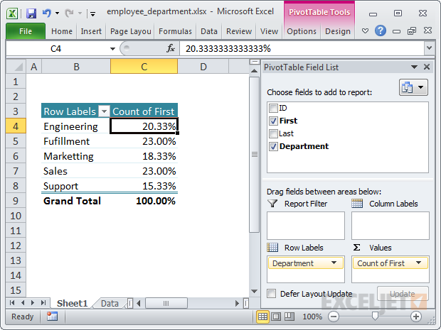
Employee breakdown by department
7.
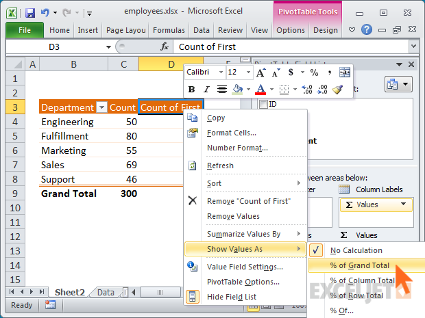
For example, perhaps you want to show a breakdown of sales by product.
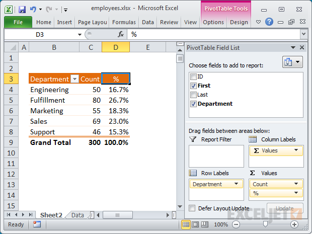
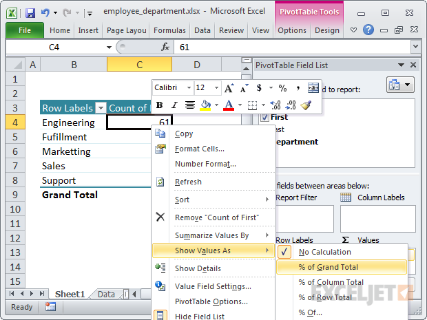
Changing value display to % of total
The sum of employees displayed as % of total
8.

Video:How to make a self-contained pivot table
10.
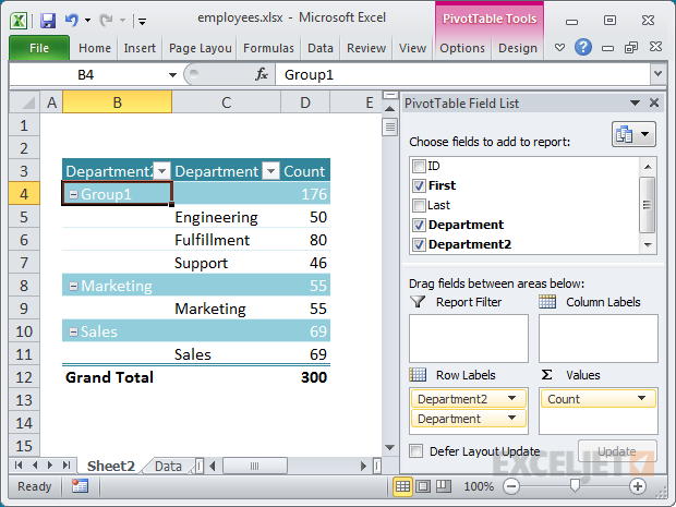
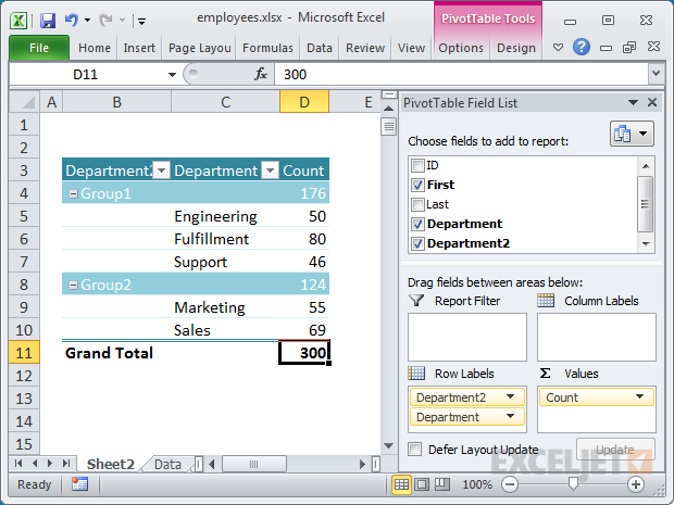
For example, assume you have a pivot table that shows a breakdown of employees by department.
Group 1 and Group 2 don’t appear in the data, they are your own custom groups.
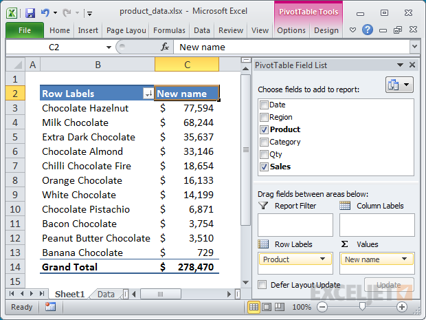
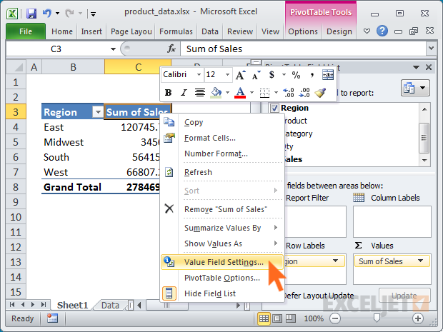
For example, you’ll see Sum of Sales, Count of Region, and so on.
However, you’ve got the option to simply overwrite this name with your own.
Just grab the cell that contains the field you want to rename and bang out a new name.

Rename a field by typing over the original name
13.
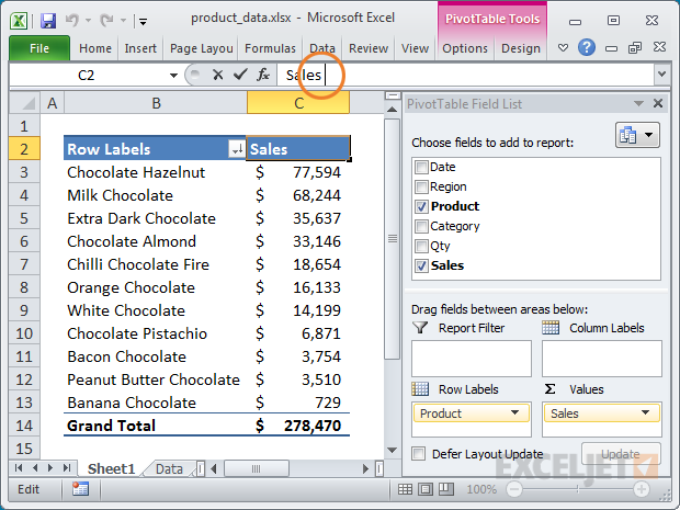
For example, suppose you have a field called Sales in your source data.
you might’t see a difference, and Excel won’t complain.

Adding a space to the name avoids the problem
14.
For example, suppose you have a pivot table that shows a count of employees by department.
The count works fine, but you also want to show the count as a percentage of total employees.

For example, assume a pivot table that shows a breakdown of sales by Region.
For example, assume you are looking at a pivot table that shows employee count by department.
You could of course just rearrange your existing pivot table to create the new view.
There are two easy ways to clone a pivot table.
The first way involved duplicating the worksheet that holds the pivot table.
Another way to clone a pivot table is to copy the pivot table and paste it somewhere else.
Using these approaches, it’s possible for you to make as many copies as you like.
When you clone a pivot table this way, both pivot tables share the samepivot cache.
Video:How to clone a pivot table
18.
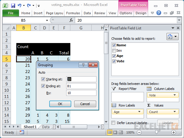
When pivot tables share the same pivot cache, they also share field grouping as well.
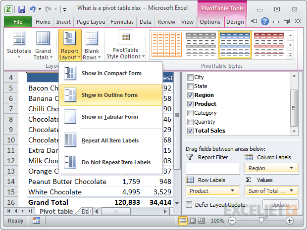
Get rid of useless headings
The default layout for new pivot tables is the Compact layout.
This layout will display “Row Labels” and “Column Labels” as headings in the pivot table.
These aren’t the most intuitive headings, especially for people who don’t often use pivot tables.
Clicking this button will disable headings completely.
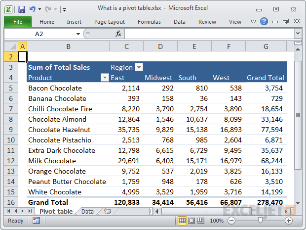
Add a little white space around your pivot tables
This is just a simple design tip.
All good designers know that a pleasing design requires a little white space.
White space just means empty space set aside to give the layout breathing room.
This will give your pivot table some breathing room and create a better looking layout.
In most cases, I also recommend that you turn off gridlines on the worksheet.
A little white space makes your pivot tables look more polished
Inspiration:5 pivot tables you haven’t seen before.
you might remove grand totals for both rows and columns
22.
By default, empty cells will display nothing at all.
To set your own character, right-click inside the pivot table and select Pivot Table options.
Keep in mind that this setting respects the applied number format.
Empty cells set to display 0 (zero) and Accounting number format gives you hyphens
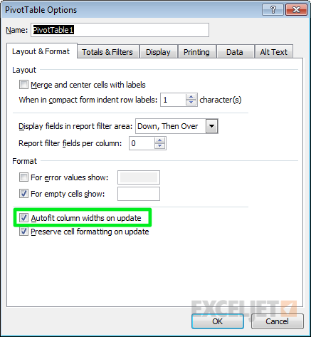
23.
To disable this feature, right-click inside the pivot table and choose PivotTable Options.
Pivot table column autofit option for Windows
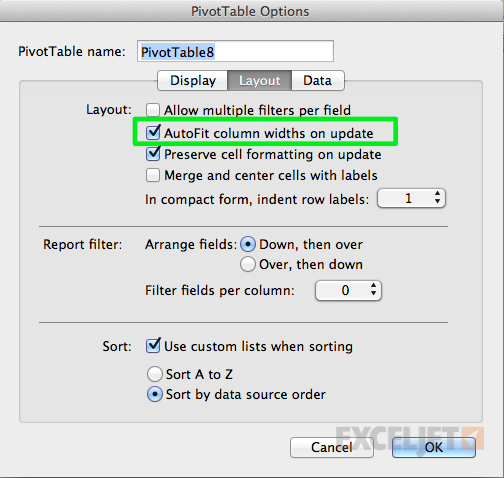
Pivot table column autofit option for Mac
Need to learn Pivot Tables?
We havesolid video trainingwith practice worksheets.