For a very long time, Excel introduced new functions at a leisurely pace.
Every few years, a handful of new functions would appear, most aimed at technical and edge-case problems.
Most users greeted these new functions with a yawn, if they noticed at all.

You might not know it, but Excel now has nearly 50 new functions!
At the same time, Microsoft overhauled Excel’s formula engine to handle array formulas natively.
Need a list of unique values from 10,000 rows?
The UNIQUE function will do it in one step.
Want to display all orders over $100?
With the new FILTER function.
Even better, because these are formulas, results are dynamic.
When data changes, you see the latest immediately.
This is not your Dad’s Excel anymore.
Many complicated formulas will become obsolete, replaced by compact and elegant alternatives.
If you use Excel frequently, this is a change you should understand and embrace.
Here’s how it works.
For the advanced Excel user, this function is amajorupgrade.
REGEXEXTRACT not only saves time but also reduces errors created by complicated workarounds.
Learn more about the REGEXEXTRACT function.

REGEXREPLACE function
The REGEXREPLACE function replaces text matching a specific regex pattern in a given text string.
you might think of REGEXREPLACE as a much more powerful version of the simplistic SUBSTITUTE function.
This function is a major upgrade to Excel’s rather primitive text-replacement functions.

Learn more about the REGEXREPLACE function.
REGEXTEST function
REGEXTEST brings the power of regular expressions to ordinary Excel formulas.
It tests whether a text string matches a specific pattern, returning TRUE or FALSE.

REGEXTEST opens up new possibilities for data validation and text analysis directly within Excel formulas.
Learn more about the REGEXTEST function.
Learn more about the GROUPBY function.

PIVOTBY function
Like the GROUPBY function, PIVOTBY can create a Pivot Table with a formula.
It’s an excellent tool for creating dynamic, formula-based summaries that update automatically when source data changes.
Learn more about the PIVOTBY function.

PERCENTOF function
PERCENTOF calculates the percentage of a subset of data relative to all data.
This function is useful in any scenario where it’s crucial that you express a part-to-whole relationship.
Learn more about the PERCENTOF function.

The concept may seem abstract, but in practice, BYCOL is quite useful.
For instance, assume you have 6 columns of numbers in C5:H14.
BYCOL runs on every column, returning a single result for each.

Since it can apply custom LAMBDA logic, BYCOL can perform operations far beyond simple sums or averages.
Learn more about the BYCOL function.
BYROW function
BYCOL is the companion to the BYROW function.

If BYROW is given an array with 100 rows, BYROW will return 100 results.
The calculation performed on each row is flexible.
The result is all 9 maximum values in one step.

BYROW runs on each row, returning a single result for each.
Learn more about the BYROW function.
CHOOSECOLS function
CHOOSECOLS selects specific columns from an array or range by position.

The columns to return are provided as numbers.
CHOOSECOLS is particularly useful when working with structured data where row positions have specific meanings.
One interesting use of CHOOSECOLS is to create amini-dashboard.
The result from CHOOSECOLS is always a single array that spills onto the worksheet.
Learn more about the CHOOSECOLS function.
CHOOSEROWS function
CHOOSEROWS works like theCHOOSECOLSfunction.

However, whereas CHOOSECOLS fetches specific columns, CHOOSEROWS fetches specific rows.
The result from CHOOSEROWS is always a single array that spills onto the worksheet.
Learn more about the CHOOSEROWS function.

Rows and columns can be dropped from the start or end of the given array.
Learn more about the DROP function.
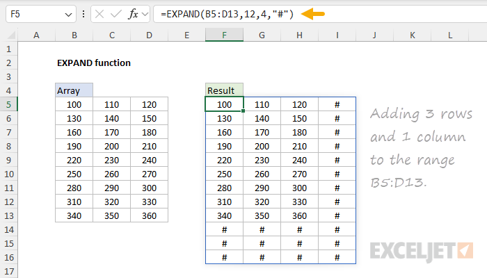
Learn more about the EXPAND function.

As implied by the name, FIELDVALUE returns a specific field value from a Data pop in.
FIELDVALUE is an alternative to the “dot” syntax: =A1.
[Previous close].

Learn more about the FIELDVALUE function.
HSTACK function
HSTACK combines arrays or ranges horizontally into a single array.
Each subsequent array is appendedto the rightof the previous array.

The output from HSTACK is fully dynamic.
If data changes, the result from HSTACK will be updated immediately.
HSTACK is closely related toVSTACK.

Use HSTACK to combine ranges horizontally and VSTACK to combine ranges vertically.
Learn more about the HSTACK function.
Of course, you could manually insert an image into a cell anytime, so why use IMAGE?

Learn more about the IMAGE function.
ISOMITTED function
ISOMITTED is a specialized function designed to work with LAMBDA functions.
Its purpose is to provide a way to make LAMBDA arguments optional.

ISOMITTED checks whether an optional argument in a LAMBDA function has been provided or not.
Inside the LAMBDA, ISOMITTED checks for b.
If b is omitted, the formula returns a+ 10.

If b is provided, the formula returns a + b.
Learn more about the ISOMITTED function.
For example, you could create a simple squaring function with =LAMBDA(x,x^2).

Once defined and named, a LAMBDA function can be used anywhere in your workbook.
LAMBDA functions can also appear inside many other new functions (i.e.
BYCOL, BYROW, MAP, SCAN, REDUCE, etc.)

that loop over arrays and apply calculations.
Learn more about the LAMBDA function.
MAKEARRAY function
MAKEARRAY is a custom array generator.

It creates an array with specified dimensions, filling it with values defined by a custom LAMBDA formula.
It’s particularly handy when you need arrays with calculated values that follow a specific pattern or rule.
Note the relatedRANDARRAYfunction can create a custom-sized array containing random numbers.

Learn more about the MAKEARRAY function.
MAP function
MAP brings a fundamental concept from functional programming to Excel.
It applies a custom operation to each cell in a range, and returns an array of results.

It’s a bit like a custom mini-function that runs on every cell.
Normally, functions like this break array formulas because they aggregate multiple values into a single value.
However, because MAP operates on one cell at a time, it works.

Learn more about the MAP function.
Learn more about the REDUCE function.
SCAN is similar toREDUCE, but instead of producing a single result, it returns anarray of intermediate results.

It’s like getting the play-by-play of a cumulative calculation at each step.
Learn more about the SCAN function.
Note that STOCKHISTORY only returns historical information recorded after the market closes.

It does not return real-time data.
Learn more about the STOCKHISTORY function.
It’s like a data slicer for ranges.

TAKE is also great for creating dynamic ranges that adjust based on the data.
Note that the TAKE function is related to theDROP function, whichremovesrows and/or columns from a range.
Learn more about the TAKE function.

It’s designed to work with structured text with a clear pattern and delimiter.
Compared to older, more complicated solutions, TEXTAFTER greatly simplifies the process of splitting text strings.
Learn more about the TEXTAFTER function.

TEXTBEFORE function
TEXTBEFORE is the counterpart toTEXTAFTER.
It extracts the portion of a string that comesbefore a specified delimiter.
TEXTBEFORE can be configured to extract text after a specific instance of a delimiter (i.e.

after the second space).
it’s possible for you to even use TEXTBEFORE together with TEXTAFTER to perform more specific text extraction.
Like TEXTAFTER, it offers options for handling multiple delimiters and case sensitivity.

Learn more about the TEXTBEFORE function.
The output from TEXTSPLIT is an array that will spill into multiple cells in the workbook.
Learn more about the TEXTSPLIT function.

TOCOL function
TOCOL transforms a two-dimensional array into a single column.
It’s like flattening your datavertically.
Learn more about the TOCOL function.

TOROW function
TOROW is the horizontal counterpart toTOCOL.
It transforms a two-dimensional array into a single row, essentially flattening datahorizontally.
Like TOCOL, it offers options to scan by row or column and can ignore blanks or errors.

Learn more about the TOROW function.
But what if you want to show this syntax directly on the worksheet?
ARRAYTOTEXT is a utility function that lets you format the values in a range in array syntax.

It converts an array or range into a text string that can be displayed directly on the worksheet.
Learn more about the ARRAYTOTEXT function.
into their text representations.

By default, text values pass through unaffected, while other values are quoted.
However, in strict mode, text values are enclosed in double quotes ("").
Learn more about the VALUETOTEXT function.

VSTACK function
VSTACK is the vertical counterpart to theHSTACKfunction.
While HSTACK stacks rangeshorizontally, VSTACK stacks rangesvertically,one on top of another.
It is also handy when you want to attach headers to calculation results inside a formula.

VSTACK can handle ranges of different widths, making it a flexible way to handle different data combination scenarios.
The output from VSTACK is dynamic and will immediately update if source data changes.
Learn more about the VSTACK function.
WRAPCOLS function
WRAPCOLS takes a one-dimensional array (i.e.
a single row or column) and wraps it into multiple columns based on a specified number of rows.
WRAPCOLS is useful when you gotta reshape linear data into a table working “by column”.

It can also be used to re-wrap data previously unwrapped by theTOCOLorTOROWfunction.
Learn more about the WRAPCOLS function.
WRAPROWS function
WRAPROWS is the row-wise version ofWRAPCOLS.

It takes a one-dimensional array (i.e.
a single row or column) and wraps it into multiple rows based on a specified number of columns.
Learn more about the WRAPROWS function.

The result from FILTER is an array of matching values from the original data.
The results from FILTER are dynamic.
If source data changes or if conditions are modified, FILTER will return new results.

This makes FILTER an excellent way to isolate and inspect specific data without altering the original dataset.
FILTER is highly versatile.
FILTER can even filter columns.

Learn more about the FILTER function.
LET function
LET brings local variables to Excel formulas.
These variables are temporary and live only in your formula.

LET can significantly improve performance by eliminating redundant calculations.
LET can radically simplify more complex formulas that reuse intermediate results or ranges multiple times.
Learn more about the LET function.
RANDARRAY function
RANDARRAY is an on-demand random number generator.
It creates an array of random numbers with specified dimensions.
RANDARRAY is useful for random sorts, random sampling, and for creating test data from randomly selected values.
Learn more about the RANDARRAY function.
SEQUENCE function
SEQUENCE is a function for generating sequential numbers.
SEQUENCE has options for the dimensions of the final array, and for the start value and step size.
Learn more about the SEQUENCE function.
SORT function
SORT brings the power of sorting directly into your formulas.
It can sort data in ascending or descending order and can sort by more than one column.
The result is a dynamic array that updates automatically when source data changes.
Learn more about the SORT function.
This means you could sort using values that don’t appear in the final result.
Like the simpler SORT function, SORTBY can sort by more than one column in ascending or descending order.
This function is especially useful when you gotta sort data in acustom order.
Learn more about the SORTBY function.
UNIQUE function
The UNIQUE function is another game-changer, making many complex formulas of the past obsolete.
As the name suggests, UNIQUE extracts a list of unique values from a range or array.
It can also be used to generate the values used in dropdown lists.
Learn more about the UNIQUE function.
XLOOKUP function
XLOOKUP is a modern successor to VLOOKUP and HLOOKUP.
It is a flexible and versatile function that can be used in a wide variety of situations.
Note: if you after multiple results, see theFILTERfunction.
Learn more about the XLOOKUP function.
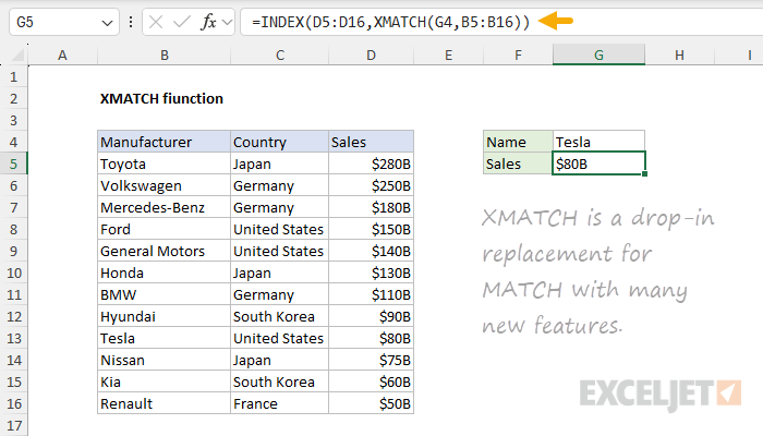
XMATCH function
XMATCH is the modernized version of the MATCH function.
Learn more about the XMATCH function.
New 2019 functions
CONCAT function
CONCAT is a modernized version of the CONCATENATE function.
Like CONCATENATE, it can join text from multiple cells without a delimiter.
For these reasons, I recommend you ignore CONCAT and use theTEXTJOIN functioninstead, which is far more capable.
Learn more about the CONCAT function.
IFS function
IFS simplifies the process of testing multiple conditions in Excel.
It allows you to evaluate several logical tests and return a value corresponding to the first TRUE result.
Think of it as a more efficient alternative to nested IF statements.
IFS makes complex conditional logic more readable and manageable.
Learn more about the IFS function.
MAXIFS function
MAXIFS finds the largest value among cells that meet multiple criteria.
It’s like combining the MAX function with multiple condition checks.
MAXIFS is a handy tool for all kinds of data analysis.
Learn more about the MAXIFS function.
MINIFS function
MINIFS is the counterpart toMAXIFS, finding the smallest value that meets multiple criteria.
Like MAXIFS, it combines the functionality of MIN with conditional filtering.
Learn more about the MINIFS function.
SWITCH function
SWITCH is like a streamlined IF-THEN-ELSE statement for Excel.
It compares a single expression against a list of values and returns the result corresponding to the first match.
Unrecognized ratings default to “???”.
Learn more about the SWITCH function.
TEXTJOIN function
TEXTJOIN is the sophisticated cousin ofCONCAT.
Because TEXTJOIN can ignore empty cells, it is more versatile than the CONCAT function.
This function is particularly useful for creating comma-separated lists and other delimited text strings.
Learn more about the TEXTJOIN function.
