Explanation
This is a standard “exact match” VLOOKUP formula with one exception: the column index is calculated using the COLUMN function.
When the COLUMN function is used without any arguments, it returns a number that corresponds to the current column.
In this case, the first instance of the formula in column E returns 5, since column E is the 5th column in the worksheet.

We don’t actually want to retrieve data from the 5th column of the customer table (there are only 3 columns total) so we need to subtract 3 from 5 to get the number 2, which is used to retrieve Name from customer data:
When the formula is copied across to column F, the same formula yields the number 3:
As a result, the first instance gets Name from the customer table (column 2), and the 2nd instance gets State from the customer table (column 3).
you’re able to use this same approach to write one VLOOKUP formula that you’re able to copy across many columns to retrieve values from consecutive columns in another table.
With two-way match
Another way to calculate a column index for VLOOKUP is to do atwo-way VLOOKUP using the MATCH function.

With this approach, the MATCH function is used to figure out the column index needed for a given column in the second table.
Related formulas
Join tables with INDEX and MATCH
VLOOKUP two-way lookup
VLOOKUP calculate grades
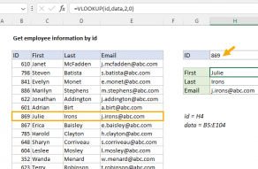
Get employee information with VLOOKUP
VLOOKUP without #N/A error
Related functions
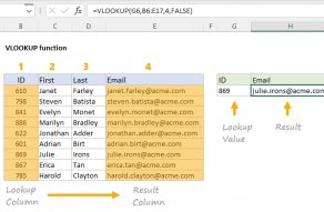
VLOOKUP Function
The Excel VLOOKUP function is used to retrieve information from a table using a lookup value.
The lookup values must appear in thefirstcolumn of the table, and the information to retrieve is specified bycolumn number.

VLOOKUP supports approximate and exact matching…
Related videos
How to use VLOOKUP to merge tables
How to use VLOOKUP
How to replace nested IFs with VLOOKUP
How to use VLOOKUP for approximate matches
Why VLOOKUP is better than nested IFs