If so, we return the predicted tide level, using thenamed rangepred.
Notice we do not provide a “value if false” for either IF.
That means if either logical test is FALSE, the outer IF will return FALSE.

For more information on nested IFs,see this article.
This is what makes this an array formula we are processing many values at once.
The other values have been replaced with FALSE.

The array above is returned directly to theMIN function.
This is anarray formulasand must be entered with control + shift + enter.
This can be done with anINDEX and MATCHformula.

When these arrays are multiplied by one another, the TRUE FALSE values are coerced to 1s and 0s.
MATCH locates the 1, and returns a position of 88 directly to theINDEX function.
This is the date that corresponds to the lowest Monday tide level.

The only difference is that the named rangetimeis provided to INDEX instead ofdate.
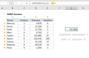
it’s possible for you to use INDEX to retrieve individual values, or entire rows and columns.
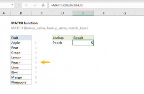
MATCH supports approximate and exact matching, andwildcards(* ?)

More than one condition can be tested by nesting IF functions.
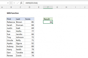
The MIN function ignores empty cells, the logical values TRUE and FALSE, and text values.
XLOOKUP supports approximate and exact matching, wildcards (* ?)