In addition, we also want to get the corresponding date.
All data is in anExcel Tablecalleddata,in the range B5:C16.
This information represents the low temperature in Fahrenheit (F) for the dates as shown.

There are several ways to solve this problem, as explained below.
XLOOKUP function
A simple solution is to use theXLOOKUP functionwithBoolean logic.
In this particular example, wecoulduse TRUE instead of 1.

Thedouble negative(–) is a simple way to perform this conversion.
The two values in row 6spillinto cells E5 and F5 as shown.
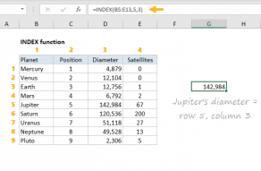
Also note thatcolumn_numinside INDEX is given as 0, to cause theINDEX functionto returnan entire rowof data (i.e.

both Date and Low).
Note: this is anarray formulathat must be entered with Control + Shift + Enter inLegacy Excel.
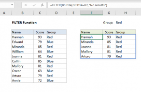
With this configuration, FILTER returns the 3 rows indatathat have negative values in the Low column.
Note that the result from FILTER includes both columns, Date and Low.
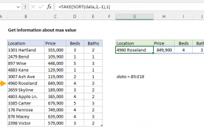
This data is returned directly to the TAKE function as thearrayargument, withrowgiven as 1.
TAKE then returns just row 1 from the matching data as a final result.

TAKE is a new function currently still inbeta.
XLOOKUP supports approximate and exact matching, wildcards (* ?)
The output from FILTER is dynamic.

If source data or criteria change, FILTER will return a new set of results.
The number of rows and columns to return is provided by separaterowsandcolumnsarguments.
Rows and columns can be extracted from the start or end of the given array.
you’re able to use INDEX to retrieve individual values, or entire rows and columns.
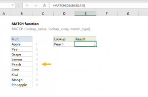
MATCH supports approximate and exact matching, andwildcards(* ?)
Often, MATCH is combined with the…