Explanation
This is a more advanced formula.
For basics, seeHow to use INDEX and MATCH.
Just select an expression in the formula bar, and press F9.

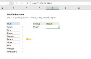
The MATCH function returns 3 to INDEX:
and INDEX returns a final result of $17.00.
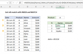
Array visualization
The arrays explained above can be difficult to visualize.
The image below shows the basic idea.
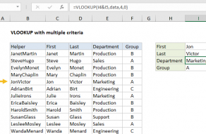
Columns B, C, and D correspond to the data in the example.
Column F is created by multiplying the three columns together.
It is the array handed off to MATCH.
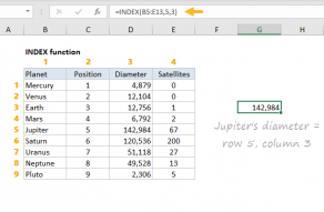
To do this, INDEX is configured with zero rows and one column.
Why would you want the non-array version?
So, a non-array formula is more “bulletproof”.
However, the tradeoff is a more complex formula.
Note: InExcel 365, it is not necessary to enter array formulas in a special way.
you might use INDEX to retrieve individual values, or entire rows and columns.
MATCH supports approximate and exact matching, andwildcards(* ?)