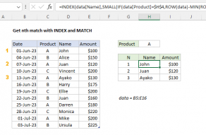
The INDEX and MATCH formula explained here is meant forlegacy versions of Excelthat do not provide the FILTER function.
However, with some effort, you’re free to make INDEX and MATCH return all matches.
This makes it much easier to identify and extract multiple matches.
Both logical tests must return TRUE in order for AND to return TRUE.
Then the value remains the same until the next match is found.
FALSE results add nothing and TRUE results add 1.

This is where the cleverness of the formula becomes apparent.
By design, each “first value” corresponds to the correct row in the data table.
If so, the INDEX/MATCH logic is run.
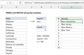
If not, IF outputs anempty string("").
Note: the extraction area needs to be manually configured to handle as much data as needed (i.e.
5 rows, 10 rows, 20 rows, etc.).
In this example, it is limited to 5 rows only to keep the worksheet compact.
I learned this technique inMike Girvin’sbookControl + Shift + Enter.
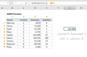
you might use INDEX to retrieve individual values, or entire rows and columns.
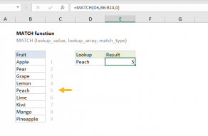
MATCH supports approximate and exact matching, andwildcards(* ?)
AND returns TRUEonly if all the conditions are met.
If any conditions are not met, the AND function returns FALSE.

These values can be numbers, cell references, ranges, arrays, and constants, in any combination.
SUM can handle up to 255 individual arguments.
Related videos
How to look things up with INDEX and MATCH


