The formula in L12 is:
The formulas in L8:L10 are for additional explanation only.
They show how the problem can be broken down into intermediate steps.
In column B, the range B5:B25 contains points.

The formula will ultimately need to return a number from this range as the final result.
In row 4, the range C4:I4 contains age ranges.
Finally, the range C5:I25 contains lift data.
These named ranges are for convenience only, to make the formula easier to read and write.
Complications
This problem is notable because the configuration is “backwards” from what is usually expected.
Finally, the ages in row 4 are text strings, whereas the age in L5 is numeric.
This too is complicated.
The trick is to extract just column 3 (age range 27-31) before we look up the lift.
We now have what we need to finally look up the lift.
Thelookup_arrayis created with the code explained above.
How can we do that?
This is actually the easiest step in the problem.
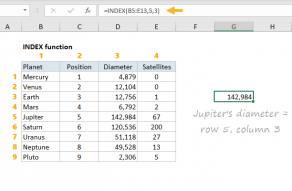
you could use INDEX to retrieve individual values, or entire rows and columns.
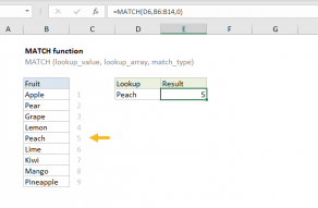
MATCH supports approximate and exact matching, andwildcards(* ?)
For example, =LEFT(“apple”,3) returns “app”.