This problem can be easily solved by applying conditional formatting with a formula based on the TEXT function.
The dropdown menu is implemented withdata validation.
TEXT function
TheTEXT functionreturns a number formatted as text, using thenumber formatprovided.
We can use the abbreviated day name for each date to match against the target date in F5.
When the result from TEXT is different, the formula will return FALSE.
This is what we need to trigger a conditional formatting rule.
Define the rule
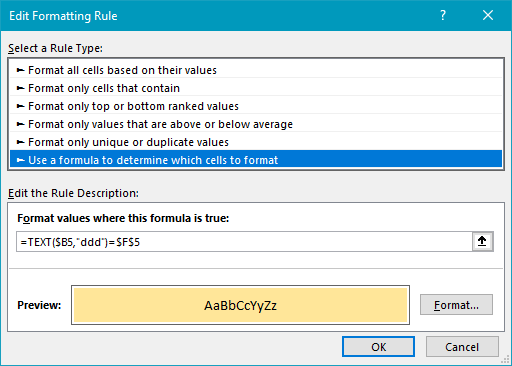
The next step is to define the conditional formatting rule itself.
With the range B5:C16 selected, navigate to Home > Conditional Formatting > New rule.
Then select “Use a formula to determine which cells to format”.
in a text string with the number format of your choice.


