The result is a dynamic summary table created with a single formula.
The output from the GROUPBY function is similar to the output from a Pivot Table, but without formatting.
The summary returned by the GROUPBY function is fully dynamic and will immediately recalculate when source data changes.
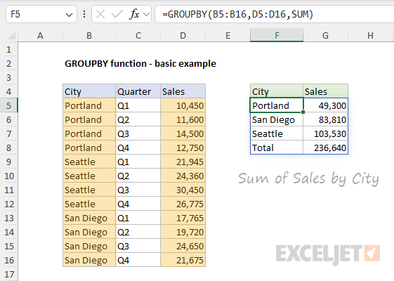
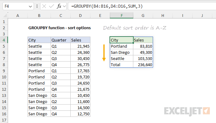
In the worksheet below, we use the GROUPBY function to summarize Sales by City.
Instead, we have manually entered a header row in F4:G4.
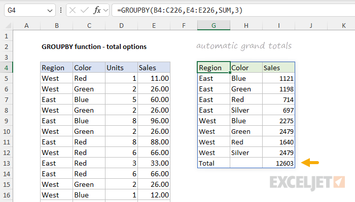
Also note that GROUPBY includes a Total row by default.
The are five possible values for field_headers:
Thefield_headerargument is optional.
Whenfield_headeris omitted, GROUPBY will automatically detect headers in the source data by testing values.
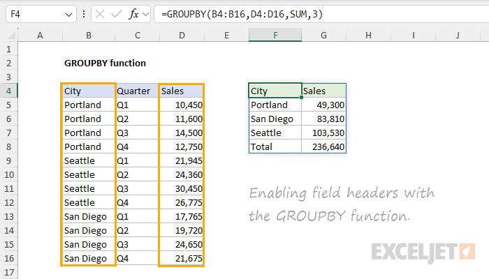
However, automatic detection only prevents the headers from being processed as values; it does not display headers.
However, the ranges used for row fields and values now include the headers in row 4.
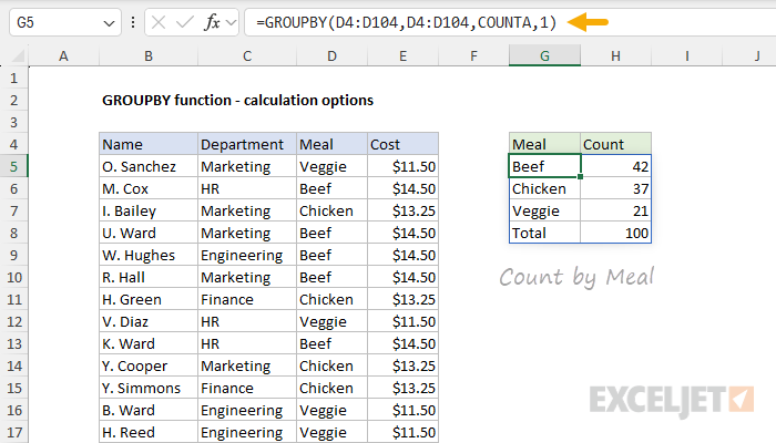
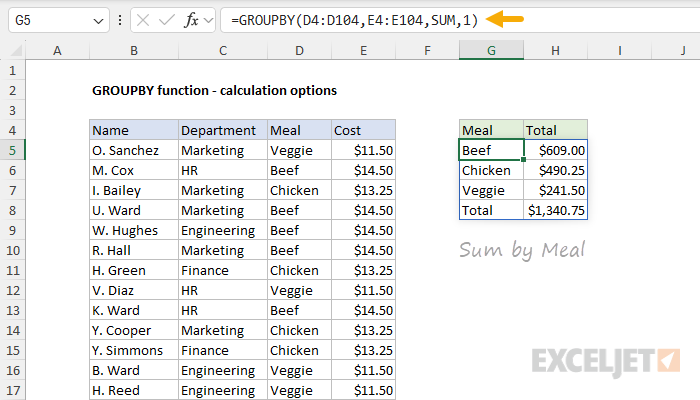
Available calculations include Excel functions like SUM, COUNT, COUNTA, MAX, MIN, etc.
The function is called witheta lambdasyntax, which is just the function name, without parentheses and arguments.
We can use the GROUPBY function to analyze this data in a variety of ways.
As a result, we provide 1 for field_headers.
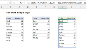
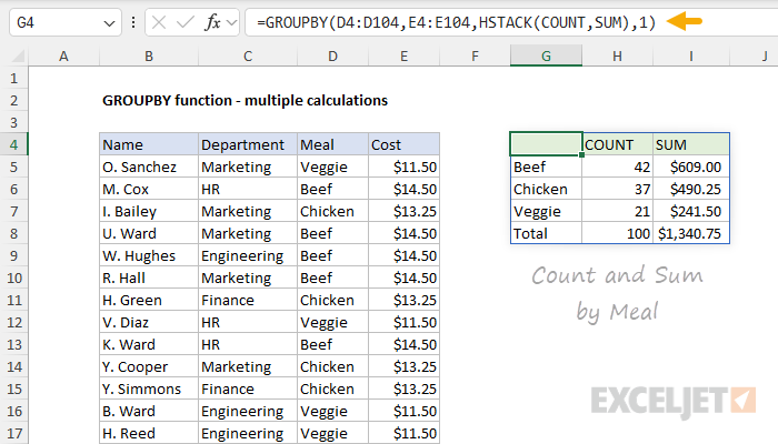
The trick is to use theHSTACK functioninside GROUPBY to call more than one function simultaneously.
This is because GROUPBY automatically adds column headers when you ask for multiple calculations.
As a result, we have COUNT in H4 and SUM in I4.
Cell G4 is blank because we have disabled field headers.
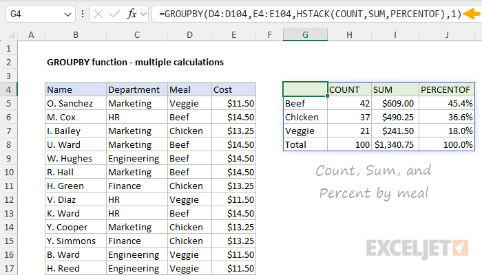
To perform another calculation, just add the function name to the values inside HSTACK.
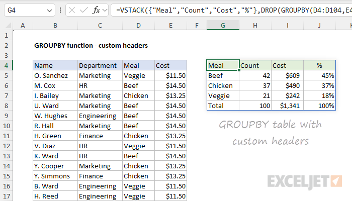
Also, note that the structure of the table is not ideal.
The first column lacks a header, and the function names used for calculations are a bit clunky.
See below for a workaround.
Depending on your use case, you may want to override these headers and supply your own custom values.
You are free to customize these values as you like.
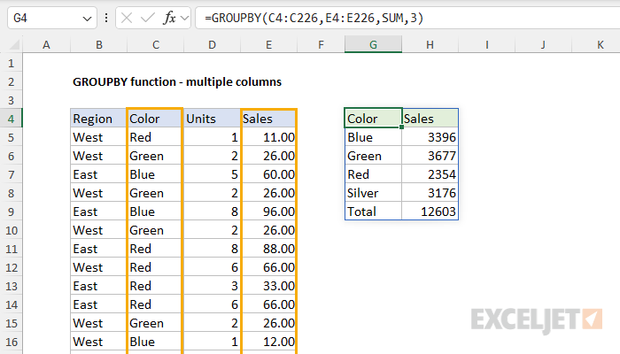
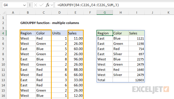
GROUPBY with multiple columns
The GROUPBY function can handle multiple columns forrow_fieldsandvaluesarguments.
When you include multiple columns, the output will have multiple row group levels.
To illustrate how this works, consider the examples below.
In the first example, we provide one column forrow_fields, and 1 column for values.
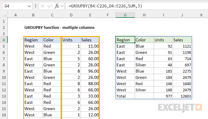
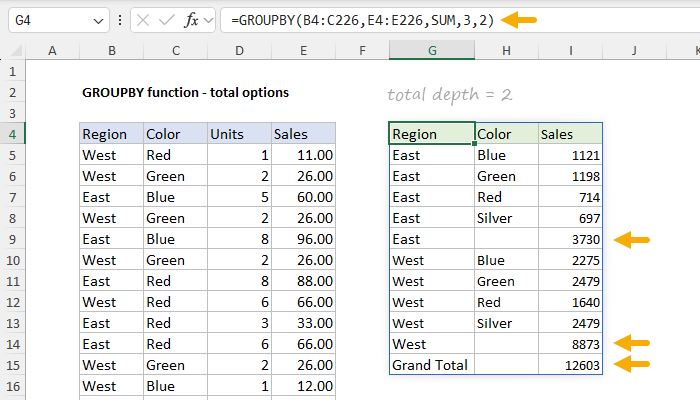
In the example below, row fields and values are provided as ranges that include two columns.
The formula in G4 is:
Here, we modified the Values range to include both Units and Sales.
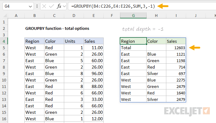
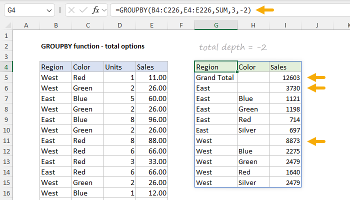
When not provided, GROUPBY will automatically display grand totals.
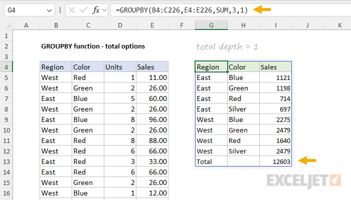
For subtotals to display,row_fieldsmust have at least 2 columns.
If you take a stab at enable subtotals whenrow_fieldscontains just one column, GROUPBY will return a #VALUE!
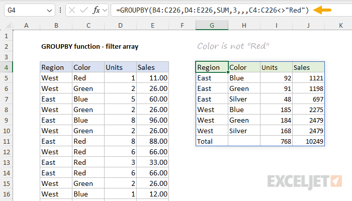
The number itself corresponds to the columns in the table, starting with 1 for the first column.
These Booleans are typically generated with a logical expression.
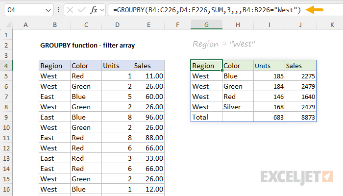
The formula in G4 looks like this:
Note thatfilter_arrayshould be the same length as the incoming data.
In the example above, we match B4:B226 to the ranges used for row and value fields.
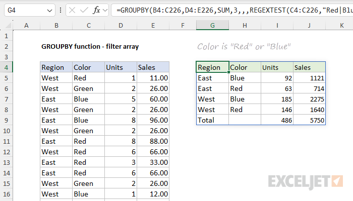
The logic can be easily modified.
For a general introduction, seeRegular Expressions in Excel.
This argument specifies the “relationship” between fields when multiple columns are provided as row fields.
There are two possible values: 0 = Hierarchy and 1 = Table.
The default value is 0 (Hierarchy).
The settingfor field_relationship affects the way sorting is handled, but only when row_fields includes multiple columns.
Whenfield_relationshipis omitted or provided as 0, the sorting of subsequent columns considers thehierarchy of earlier columns.
Whenfield_relationshipis set to 1, the sorting of each field column works independently.
I do not have a good example of field relationships in action.
If you have a good example,kindly let me know.
Why two syntax options?
The short form is for convenience.
It is concise and easy to read.
However, the behavior cannot be customized.
The long-form syntax uses the LAMBDA function and can be customized as needed to apply a more advanced calculation.
To illustrate this concept, suppose you want the round values that GROUPBY returns to the nearest 1000.
The GROUPBY function then returns the rounded sum in the final output.
A dynamic range is a range that expands and contracts as rows are added or removed.
In both cases, you will then need to feed specific columns of the range into GROUPBY.
The result is a dynamic summary table created with a single formula.
HSTACK Function
The Excel HSTACK function combines arrays horizontally into a single array.
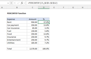
The output from PERCENTOF is a decimal number that can be formatted with Excel’s percentage number format….