In the current version of Excel, a good way to solve this problem is with the XLOOKUP function.
In older versions of Excel, you could use the LOOKUP function.
Both methods are explained below.

XLOOKUP function
TheXLOOKUP functionis a modern upgrade to the VLOOKUP function.
XLOOKUP is very flexible and can handle many different lookup scenarios.
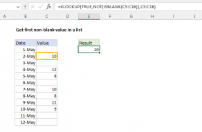
Because B5:B16 contains 12 values, the expression returns anarraythat contains 12 TRUE and FALSE results.

In this array, the TRUE values in the array indicatenon-blankcells and the FALSE values indicateblankcells.
With thereturn_arrayprovided as B5:B16, XLOOKUP returns 15-Jun-23 as a final result.
Dealing with errors
If the last non-empty cell contains an error, the error will be ignored.
For more details, seeBoolean Algebra in ExcelandXLOOKUP with multiple criteria.
One solution is to use theLOOKUP function, which can handlearray operationsnatively.
This array becomes thelookup_arrayargumentin LOOKUP.

Thelookup_valueis given as the number 2.
This may seem baffling, but there is a good reason.
We are using 2 as a lookup value to force LOOKUP to scan to theend of the data.

Since theresult_vectoris B5:B16, the final result is: 15-Jun-23.
When LOOKUP can’t find a match, it will match the next smallest value.
LOOKUP’s default behavior makes it useful for solving certain problems in Excel.

XLOOKUP supports approximate and exact matching, wildcards (* ?)
for partial matches, and lookups in vertical or horizontal ranges….


