The easiest way to do this is with the newer TEXTAFTER function.
Both options are explained below.
Note the contrast between the modern solution and the legacy solution.
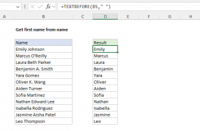
TEXTAFTER extracts text that occursaftera given delimiter.
In its simplest form, TEXTAFTER only requires two arguments, text and delimiter.
Normally, a positive instance number tells TEXTAFTER to count instances from the left.
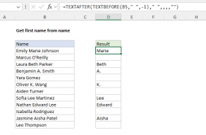
Anegativeinstance number tells TEXTAFTER to count instances from theright.
In other words, we are asking TEXTAFTER for the text after thelastspace.
TEXTAFTER has many other options that you’re able to read .

This is a complicated formula.
contains one or more middle names).
At the core, this formula uses theMID functionto extract characters in the name starting at a particular location.
Once we have that number, we simply add 1 to determine astart_numfor MID.
How does the code replace only thelastspace with an asterisk?
This is the clever part.
Buckle up, because the explanation gets a bit technical.
The key to this formula is this bit:
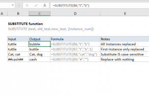
Normally, theSUBSTITUTE functionwill replace all instances ofold_textwithnew_text.
If the argument is omitted, all instances are replaced.

If a number like 2 is provided, SUBSTITUTE will replace only the second instance.
At this point, the problem becomes how to calculate the correctinstance_num.
you might find a more detailed explanationhere.

We then add 1 to get a starting position of 11.
This is the number used fornin the formula above.
Notice that we providenum_charsas 100.

This arbitrary number is part of a shortcut with MID.
you might increase this number as needed.
Note: Extra spaces in the names will cause problems with the formulas on this page.

For example, =MID(“apple”,2,3) returns “ppl”.
LEN will also count characters in numbers, but number formatting is not included.
SUBSTITUTE Function
The Excel SUBSTITUTE function replaces text in a given string by matching.
When the text is not found, FIND returns a #VALUE error.

