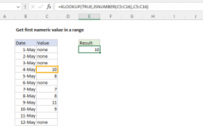
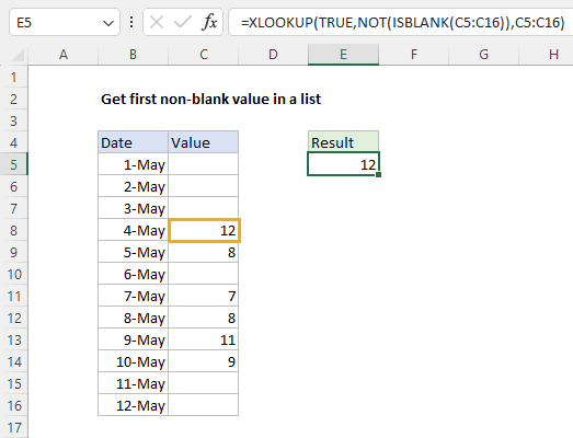
The easiest way to solve this problem is with the XLOOKUP function.
XLOOKUP function
TheXLOOKUP functionis a modern upgrade to the VLOOKUP function.
XLOOKUP is very flexible and can handle many different lookup scenarios.
For more details, seeHow to use the NOT function.
It first uses ISBLANK to create an array with TRUE for blank cells and FALSE for non-blank cells.
This final array serves as the lookup array for XLOOKUP.
The TRUE values in the array indicate blank cells, and the FALSE values indicate non-blank cells.
The array is returned directly to the NOT function so that “reverse” the results.
Testing the formula
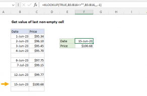
To test the formula, we can delete the value in C6.
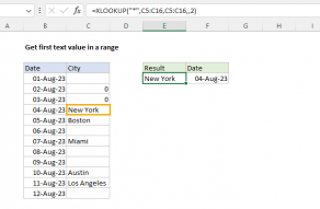
This formula has basically the same logic as the XLOOKUP formula above.
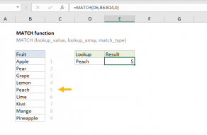
The MATCH function is used to find the position of the first non-blank cell in C5:C16.
For more details, seeHow to use INDEX and MATCH.
XLOOKUP supports approximate and exact matching, wildcards (* ?)
When given TRUE, NOT returns FALSE.
When given FALSE, NOT returns TRUE.
Use the NOT function to reverse a logical value.
For example, if A1 contains “apple”, ISBLANK(A1) returns FALSE.
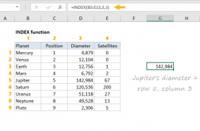
it’s possible for you to use INDEX to retrieve individual values, or entire rows and columns.
MATCH supports approximate and exact matching, andwildcards(* ?)
Often, MATCH is combined with the…