See below for a detailed explanation of both approaches.
For convenience,id(H4) anddata(B4:E104) arenamed ranges.
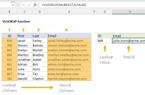
VLOOKUP function
VLOOKUP is an Excel function to get data from a table organizedvertically.

Lookup values must appear in the first column of the table passed into VLOOKUP.
Notice that this is theonly thing changingin the formulas above, every other input remains the same.
Finally, we have the last value, which is zero (0).

We use zero in these formulas to tell VLOOKUP to only perform an exact match.
In “exact match mode” VLOOKUP will only match an id value exactly.
If an id is not found, VLOOKUP will return the #N/A error.

The named ranges will behave likeabsolute referencesand will not change when the formula is copied to a new location.
Note: VLOOKUP will perform an approximate match by default.
This minimal syntax for XLOOKUP looks like this:
Unlike VLOOKUP, we don’t give XLOOKUP theentire table.

Instead, we provide separate ranges forlookup_arrayandreturn_array.
The value for lookup_value is the named rangeid(H4).
However, in the example shown, we only have the named rangedata(B5:E104).
Is there a way to use the entire table directly with XLOOKUP?
It’s a little tricky, but we can use the CHOOSECOLS function.
Note: Excel purists will point out that we could also use theINDEX functionto retrieve columns for XLOOKUP.

XLOOKUP supports approximate and exact matching, wildcards (* ?)
The columns to return are provided as numbers in separate arguments.
Each number corresponds to the numeric index of a column in the given array.

TAKE Function
The Excel TAKE function returns a subset of a given array.
The number of rows and columns to return is provided by separaterowsandcolumnsarguments.
Rows and columns can be extracted from the start or end of the given array.

The number of rows and columns to remove is provided by separaterowsandcolumnsarguments.


