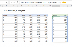
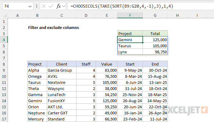
We also want to remove unnecessary columns to create a clean, uncluttered view.
This is a useful technique for creating a simple dashboard report with a dynamic set of data.
In addition, the source data can be located on a different worksheet.
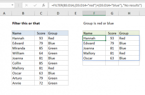
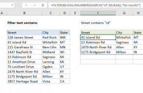
The first method uses the FILTER function to extract data of interest.
This is the best approach when the logic needed to select important data is more complex.
The second approach uses the TAKE function to grab the most important records after sorting.
This is a more powerful way to isolate important information compared to sorting only.
Note: We could sort the data before filtering with the same result.
However, using FILTER first is more efficient since we are only sorting records that meet our criteria.
This approach makes sense when sorting alone is enough to “surface” the most important data.
These techniques are useful for creating simple, dynamic summaries that update automatically as the source data changes.
In the example shown, both methods work well.
Wait, what about Pivot Tables?
Yes, you’re free to definitely solve this challenge with a Pivot Table as well.
In fact, the workbook attached to this article has a working Pivot Table on Sheet3.
Until a couple of years ago, Pivot Tables were thebestway to solve this challenge.
In contrast, a formula-based table will recalculate when any data changes.
In addition, two brand new functions,GROUPBYandPIVOTBY, directly mimic Pivot Table functionality.
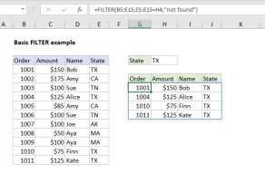
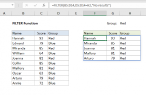
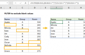
The output from FILTER is dynamic.
If source data or criteria change, FILTER will return a new set of results.
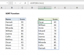
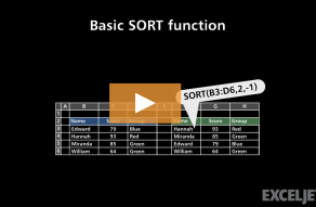
Values can be sorted by one or more columns.
SORT returns a dynamic array of results.
CHOOSECOLS Function
The Excel CHOOSECOLS function returns specific columns from an array or range.
The columns to return are provided as numbers in separate arguments.
Each number corresponds to the numeric index of a column in the given array.
TAKE Function
The Excel TAKE function returns a subset of a given array.
The number of rows and columns to return is provided by separaterowsandcolumnsarguments.
Rows and columns can be extracted from the start or end of the given array.
Related videos
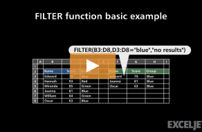
FILTER function basic example
Basic SORT function example