Once we have identified common values, we can extract a list of common values from either list.
This is because we need the resulting array from XMATCH to match the dimensions of thearrayprovided to FILTER.
The first step in this process is identifying common values.

Since the lookup item in XMATCH is most often a single value, you might find this configuration strange.
Rest assured, there is a method to this madness.
The #N/A errors represent values in B5:B16 thatwere not foundin the range D5:D14.

The numbers represent the location of values thatwere found.
For example, looking at the first four values in the array:
And so on.
However, the numbers and errors are gone.

This is exactly what we need for the FILTER function.
Values associated with 0 are removed.
However, it comes with a significant caveat: it only works on ranges.

This limitation is shared by all of the *IFs functions and isdiscussed in some detail here.
The output from FILTER is dynamic.
If source data or criteria change, FILTER will return a new set of results.

It is a more robust and flexible successor to the MATCH function.
XMATCH supports approximate and exact matching, reverse search, and wildcards (* ?)
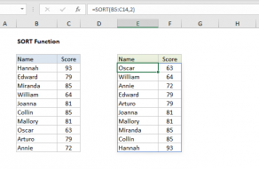
Values can be sorted by one or more columns.

SORT returns a dynamic array of results.
COUNTIF can be used to count…
Related videos
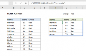
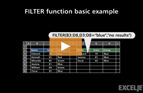
FILTER function basic example