Quick Links
Pivot tables are one of the most powerful and useful features in Excel.
If you gotta be convinced that Pivot Tables are worth your time,watch this short video.
Grab thesample dataand give it a try.
Learning Pivot Tables is a skill that will pay you back again and again.
Pivot tables can dramatically increase your efficiency in Excel.
What is a pivot table?
you’ve got the option to think of a pivot table as a report.
However, unlike a static report, a pivot table provides aninteractive view of your data.
The beauty of pivot tables is they allow you to interactively explore your data in different ways.
In this section, we’ll build several pivot tables step-by-step from a set of sample data.
With experience, the pivot tables below can be built in about 5 minutes.
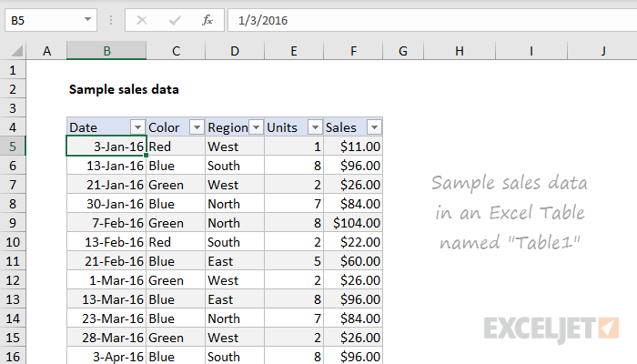
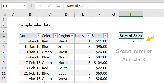
This data is perfect for a pivot table.
Data in a properExcel Tablenamed “Table1”.
Note: I know this data is very generic.
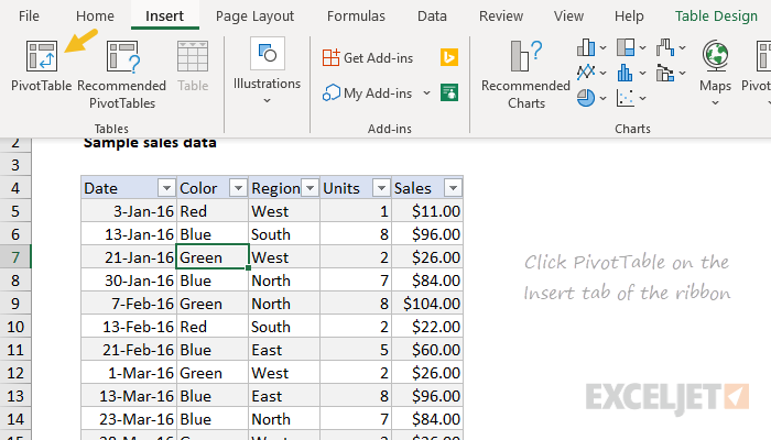
Insert Pivot Table
1.
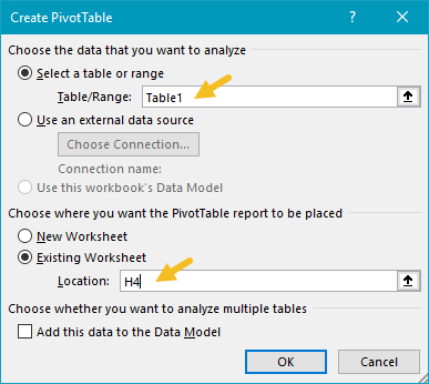
Notice the data range is already filled in.
The default location for a new pivot table is New Worksheet.
Override the default location and enter H4 to place the pivot table on the current worksheet:
3.
Click OK, and Excel builds an empty pivot table starting in cell H4.
Note: there are good reasons to place a pivot table on a different worksheet.
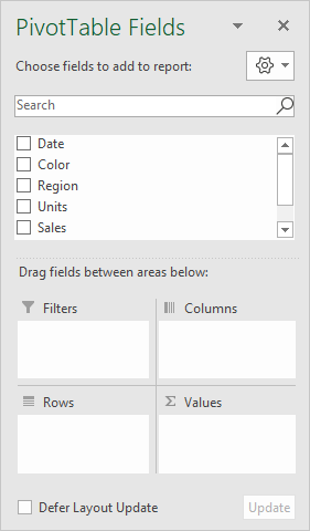
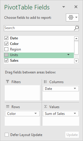
Excel also displays the PivotTable Fields pane, which is empty at this point.
The Filters area is used to apply global filters to a pivot table.
Note: the pivot table fields pane shows how fields were used to create a pivot table.
Learning to “read” the fields pane takes a bit of practice.

See below andalso herefor more examples.
Add fields
1.
Drag the Sales field to the Values area.
Excel calculates a grand total of 26356.
This is the sum of all sales values in the entire data set:
2.
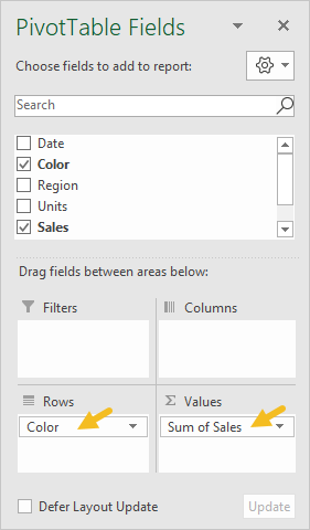
Drag the Color field to the Rows area.
Excel breaks out sales by Color.
This makes sense because we are still reporting on the full set of data.
Let’s take a look at the fields pane at this point.

This is a big time-saver when data changes frequently.
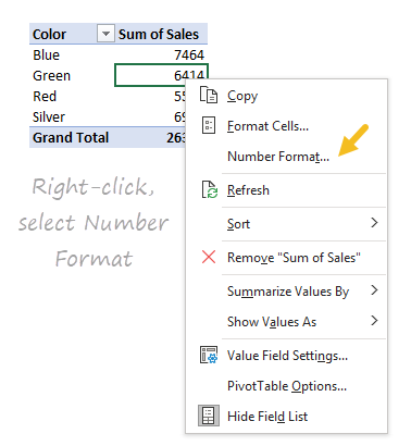
Right-click any Sales number and choose Number Format:
2.
Sorting by value
1.
Right-click any Sales value and choose Sort > Largest to Smallest.
Excel now lists top-selling colors first.
This sort order will be maintained when data changes, or when the pivot table is reconfigured.
Refresh data
Pivot table data needs to be “refreshed” so that bring in updates.
Select cell F5 and change $11.00 to $2000.
Right-click anywhere in the pivot table and select “Refresh”.

Notice “Red” is now the top-selling color, and automatically moves to the top:
3.
Change F5 back to $11.00 and refresh the pivot again.
Try changing an existing color to something new, like “Gold” or “Black”.

When you refresh, you’ll see the new color appear.
you’re able to use undo to go back to the original data and pivot.
Second value field
you could add more than one field as a Value field.

One option is to show values as a percent of the total.
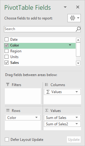
If you want to display the same field in different ways, add the field twice.
Remove the Units from the Values area
2.

Add the Sales field (again) to the Values area.
This grouping can be customized.
Remove the second Sales field (Sales2).

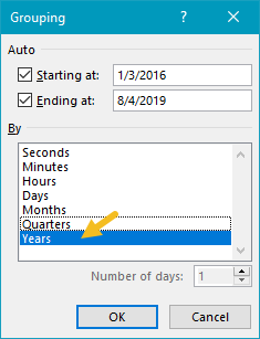
Drag the Date field to the Columns area.
Right-click a date in the header area and choose “Group”:
4.
We can guess that Silver was introduced as a new color in 2018.

Pivot tables often reveal patterns in data that are difficult to see otherwise.
Two-way Pivot
Pivot tables can plot data in various two-dimensional arrangements.
Drag the Date field out of the columns area
2.

Drag Region into the Columns area.
Excel builds a two-way pivot table that breaks down sales by color and region:
3.
Swap Region and Color (i.e.

drag Region to the Rows area and Color to the Columns area).
Each table presents a different view of thesame data, so they all sum to thesame total.
The above example shows how quickly you’re free to build different pivot tables from the same data.

you could createmany other kinds of pivot tables, using all kinds of data.
Key Pivot Table benefits
Simplicity.
Basic pivot tables are very simple to set up and customize.
There is no need to learn complicated formulas.
you’re able to create a good-looking, useful report with a pivot table in minutes.
Unlike formulas, pivot tables don’t lock you into a particular view of your data.

you’ve got the option to quickly rearrange the pivot table to suit your needs.
you’re free to evenclone a pivot tableand build a separate view.
In fact, a pivot table will often highlight problems in the data faster than any other tool.
A Pivot table can apply automatically apply consistent number and style formatting, even as data changes.
Pivot tables are designed for ongoing updates.
Pivot tables contain several tools for filtering data.

Need to look at North America and Asia, but exclude Europe?
A pivot table makes it simple.
once you nail a pivot table, you’ve got the option to easilycreate a pivot chart.
More pivot table resources


