This is a big upgrade and a welcome change.
Dynamic Arrays solve some really hard problems in Excel, and will fundamentally change the way worksheets are designed.
Once you see how they work, you’ll never want to go back.
Availability
Dynamic arrays and the new functions below are only availableExcel 365and Excel 2021.
Excel 2019 and earlierdo notoffer dynamic array formulas.
Example
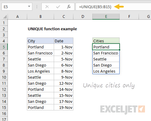
Before we get into the details, let’s look at a simple example.
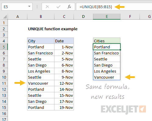
Like all formulas, UNIQUE will update automatically when data changes.
Below, Vancouver has replaced Portland on row 11.
This will immediately be more logical to formula users.
It is also a fully dynamic behavior when source data changes, spilled results will immediately update.
The rectangle that encloses the values is called the “spill range”.
You will notice that the spill range has special highlighting.
In the UNIQUE example above, the spill range is E5:E10.
When data changes, the spill range will expand or contract as needed.
You might see new values added, or existing values disappear.
In this way, a spill range is a new kind of dynamic range.
However, unless the formula is entered as amulti-cell array formula, onlyone valuewill be displayed on the worksheet.
This behavior has always made array formulas difficult to understand.
Spilling makes array formulas more intuitive.
Note: when spilling is blocked by other data, you’ll see a #SPILL error.
Once you make room for the spill range, the formula will automatically spill.
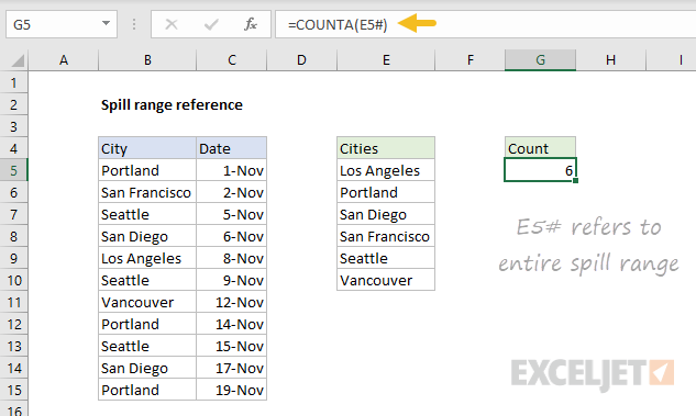
you’re able to feed a spill range reference into other formulas directly.
Massive simplification
The addition of new dynamic array formulas means certain formulas can be drastically simplified.
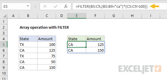
For example, below we use the FILTER function to extract records in group “A”.

This is a huge benefit for many users because it makes the process of writing formulas so much simpler.
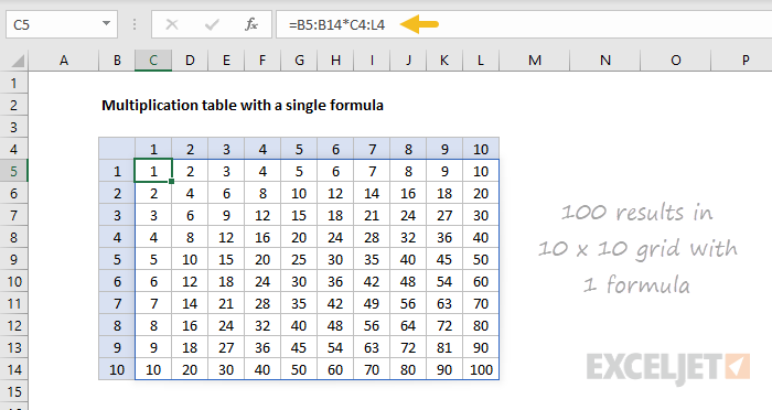
For another good example, see the multiplication table below.
Chaining functions
Things get really interesting when you chain together more than one dynamic array function.
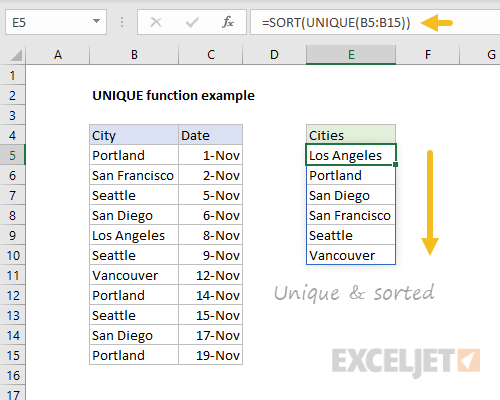
Perhaps you want to sort the results returned by UNIQUE?
This includes older functions not originally designed to work with dynamic arrays.
For example, inLegacy Excel, if we give theLEN functionarangeof text values, we’ll see asingleresult.

In Dynamic Excel, if we give the LEN function a range of values, we’ll seemultipleresults.
For instance, theVLOOKUP functionis designed to fetch a single value from a table, using a column index.
All formulas
Finally, note that dynamic arrays work withall formulasnot justfunctions.

In fact, you may see “array” and “range” used almost interchangeably.
Video:What is an array?
For a demonstration, see:How to filter with two criteria(video).
When a formula is created, Excel checks if the formula might return multiple values.
When you give a range or array to a function not programmed to accept arrays natively (i.e.
The result is an array with the same dimensions as the input array.

Lifting is a built-in behavior that happens automatically.
In Dynamic Excel, some older functions like EOMONTH “resist” spilling when provided a range.
This limitation comes from certain functions expecting a single value instead of a range.

error is essentially reporting the range as an unexpected value.
However, adding an operator in front of the reference will often fix the problem.
For example, EOMONTH(+A1:A5,1) will work and spill properly.

EOMONTH returns 5 results through the normal process of lifting, which is not function-specific.
The @ character enables a behavior known as “implicit intersection”.
Implicit intersection is a logical process where many values are reduced to one value.
In Dynamic Excel, it is not typically needed, since multiple results can spill onto the worksheet.
When it is needed, implicit intersection is invoked manually with the @ character.
In Legacy Excel, a formula that returns multiple values won’t spill on the worksheet.


