This is a tricky problem in Excel for a couple of reasons.
First, there is no direct way to generate a list of sheets in a workbook with a formula.
I recommend you place this sheet at the end of the workbook.
In the example above, the Errors sheet is the last.
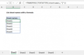
Next, we need to create a list of sheet names.
Note that the names you enter must match the sheet names exactly.

For step-by-step instructions for listing sheet names with a formula,see this article.
Power Query
Another option to automatically generate sheet names in a workbook is to use Power Query.
Instead, you must right-go for the list and click “Refresh”.

On the plus side, there is no need to save the file in a special format.
You will need to adjust this range to suit your workbook.
INDIRECT will trigger a recalculation with each change to the workbook!

This is done with theINDIRECT function, which is designed to convert a text string into a valid reference.
For example:
The main thing to understand is each reference above begins as plain text.
INDIRECT evaluates the text and converts it to a valid cell reference that can be used in a formula.

Note we are carefully adding single quotes (') around the sheet name.
These are required when a sheet name contains space or punctuation.
We also need to add an exclamation point (!)

Most of these values will be FALSE, since most cells in the range do not contain errors.
After this step, the vast majority of the values will be zeros.
Finally, we are ready to add things up with the SUMPRODUCT function.

This sum represents the count of errors on the sheet.
As the formula is copied down, the same process is repeated for each sheet in the list.
In older versions, SUM must be entered as anarray formulawith control + shift + enter.
SeeWhy SUMPRODUCT?for more info.
The formula in cell D5, copied down, is:
HYPERLINK takes two arguments:link_locationandfriendly_name.
As before we are concatenating values together to assemble a reference to a particular sheet.
As the formula is copied down, it returns a link to each sheet in the list.
you’re able to customize the destination cell and the anchor text as desired.
Otherwise, return “Invalid reference”.
TheISREF functionis used to test the reference returned by INDIRECT and theIF functionis used to control the flow.
INDIRECT is useful when you want to assemble a text value that can be used as a valid reference.
HYPERLINK Function
The Excel HYPERLINK function returns a hyperlink to a given destination.
you’re free to use HYPERLINK to create a clickable hyperlink with a formula.
you could use the ISREF function to check for a reference in a formula.
