Quick Links
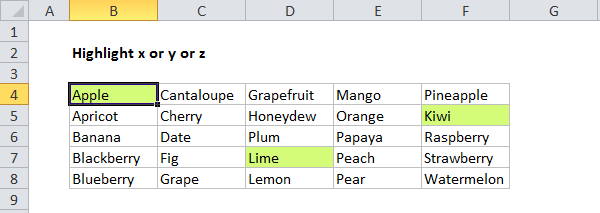
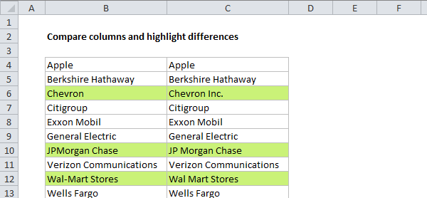
Conditional formatting is a fantastic way to quickly visualize data in a spreadsheet.
However, you’re free to also create rules with your own custom formulas.
Formulas give you maximum power and flexibility.
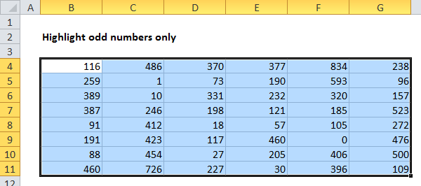
Sure, you could create a rule for each value, but that’s a lot of trouble.
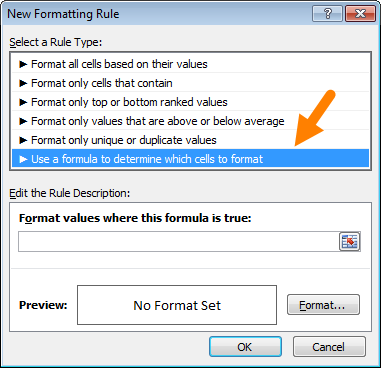
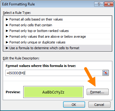
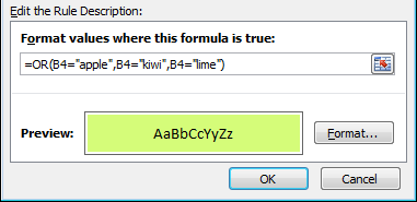
Create a conditional formatting rule, and pick the Formula option
3.
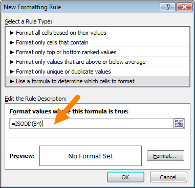
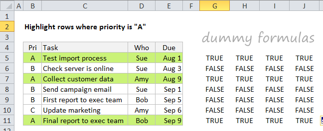
Enter a formula that returns TRUE or FALSE.
Set formatting options and save the rule.
If you struggle with this, see the section onDummy Formulasbelow.
This page hasdetails and a full explanation.
First, see to it you started the formula with an equals sign (=).
If you forget this step, Excel will silently convert your entire formula to text, rendering it useless.
This can be a big time-saver when you’re struggling to get cell references working correctly.
For a detailed explanation,see this article.
If you are trying to use an array constant, try creating a named range instead.
More CF formula resources