Explanation
This example is based on theformula explained in detail here:
The formula uses the greater thanoperator(>) to check row in the data.
On the left, the formula calculates a “current row”, normalized to begin at the number 1:
On the right, the formula generates a threshold number:
When the current row is greater than the threshold, the formula returns TRUE, triggering the conditional formatting.
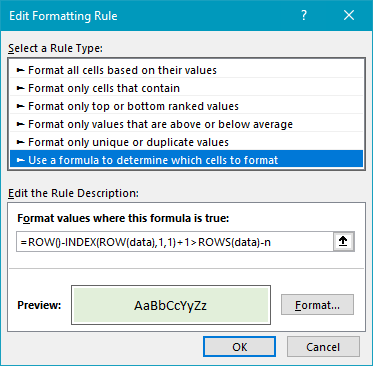
Conditional formatting rule
The conditional formatting rule is set up to use a formula like this:
With a table
you’re able to’t use a table name in a CF formula at present.
However, it’s possible for you to select or enter the table data range when creating the formula in the CF window, and Excel will keep the reference up to date as the table expands or shrinks.
Related formulas
Conditional formatting based on another cell
Highlight values between
Highlight values greater than
Highlight cells that contain
Highlight entire rows
Related videos
How to apply conditional formatting with a formula
Conditional formatting based on a different cell
How to build a search box with conditional formatting
How to highlight rows with conditional formatting
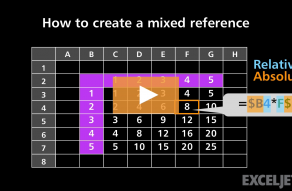
How to create a mixed reference