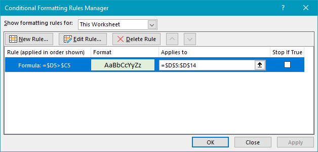
To apply conditional formatting based on a value in another column, you can create a rule based on a simple formula. In the example shown, the formula used to apply conditional formatting to the range D5:D14 is: =$D5>$C5 This highlights values in D5:D14 that are greater than C5:C14. Note that both references are mixed in order to lock the column but allow the row to change.
April 14, 2025 · 1 min · 14 words · Michelle Rodriguez
When the formula returns TRUE, the rule is triggered and the highlighting is applied.