Explanation
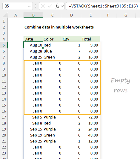
The goal is to combine data from different worksheets with a formula.
This means the solution should also provide a way to remove empty rows in the final result.
The first step is to combine the data, which is done with the VSTACK function.

However, the same approach will work with larger sets of data in many more worksheets.
When you have data in “normal” ranges (i.e.
This is the core of the formula the part that does the actual data consolidation.
This works well, as you might see in the screen below.
The reason we do this is because we are going to use the same datatwicein FILTER.
By using a variable, we only need to initiate the VSTACK operation one time.
LET function
TheLET functionallows you to name variables inside a formula.
This makes more complex formulas easier to read and write.
It also improves performance since certain operations only need to run one time.
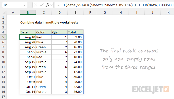
The next step is to remove the empty rows.
For that, we’ll use the FILTER function.
In this case, we are asking CHOOSECOLS for the first column indata.
Then we use alogical expressionto test for “not empty” cells in the column.
The result is an array of TRUE and FALSE values, one per row.
This array is returned to FILTER as theincludeargument.
The rows associated with FALSE values are discarded.
If you need a more robust test for empty rows,see this example.
With larger amounts of data, this will slow the formula down.
As long as this remains true, you might easily expand the 3D reference to include additional sheets.
However, there is no requirement that you use a 3D reference.
The output from FILTER is dynamic.

If source data or criteria change, FILTER will return a new set of results.
The columns to return are provided as numbers in separate arguments.
Each number corresponds to the numeric index of a column in the given array.

Related videos
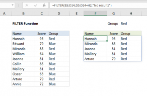
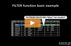
FILTER function basic example