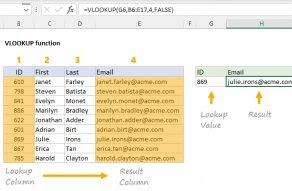
Because we are using VLOOKUP, the full name must be in the first column.
For simplicity, the table has been named “states”.
The final argument, range_lookup, has been set to zero (FALSE) to force an exact match.

VLOOKUP locates the matching entry in the “states” table, and returns the corresponding 2-letter abbreviation.
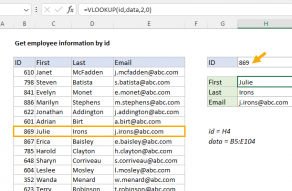
This same approach can be used to lookup and convert many other types of values.
For example, you could use VLOOKUP to map numeric error codes to human readable names.

In that case, you’ll need to switch to INDEX and MATCH.
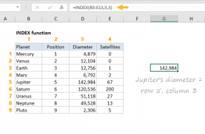
Here, we use INDEX to return whole columns by supplying a row number of zero.
you’re free to use INDEX to retrieve individual values, or entire rows and columns.
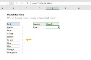
MATCH supports approximate and exact matching, andwildcards(* ?)