Formulas are the bread and butter of Excel.
If you use Excel on a regular basis, I bet you use a lot of formulas.
But crafting a working formula can take way too much time.

In this article, I share some good tips to save you time when working with formulas in Excel.
Video:20 tips to save time with Excel formulas
1.
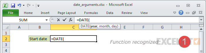
Don’t add the final parentheses to a function
Let’s start out with something really easy!
When you enter one function on its own (SUM, AVERAGE, etc.)
you don’t need to enter the final closing parentheses.
For example, you’re free to just enter:
=SUM(A1:A10
and press return.
Excel will add the closing parentheses for you.
It’s a small thing, but convenient.
Note: this won’t work if your formula contains more than one set of parentheses.
There are several ways you’ve got the option to do this.
If you’re just moving a formula to a nearby location, try drag and drop.
Dragging will keep all addresses intact and unchanged.
If you are moving a formula to a more distant location, use cut and paste.
you might then paste at a new location.
The result will be a formula identical to the original.

This will convert the formulas to text.
Now copy and paste the formulas to a new location.
After you paste the formulas, and with all formulas selected, reverse the search and replace process.

Search for the hash (#) and replace an equal sign (=).
This will restore the formulas to working order.
(Credit:Tom Urtis)
4.

The fill handle is the little rectangle that sits in the lower right corner of all selections in Excel.
Excel uses this data to figure out how far down the worksheet to copy the formula.
Just verify to grab the original formula and the target cells first.

Video:Shortcuts to move around a big list fast
5.
This saves a lot of time and also helps to prevent errors.
Note: formulas in a table will automatically use structured references (i.e.

in the example above =[@Hours][@Rate] instead of =C4D4.
However, you’re able to pop in cell addresses directly and they will be preserved.
As you punch in, you’ll see a list of “candidate” functions appear below.

This list will narrow with each letter you bang out.
On Windows, functions are selected automatically as you key in.
Use Control + click to enter arguments
Don’t like typing commas between arguments?

you’re free to have Excel will do it for you.
This will work with any function where you are supplying references as arguments.
To select arguments, work in two steps.

In step one, click to put the cursor inside the function whose argument you want to select.
Excel will then display a hint for that function that shows all arguments.
In step two, poke the argument you want to select.

Excel will pick the entire argument, even when it contains other functions or formulas.
This is a nice way to select arguments when using F9 to debug a formula.
Want to learn more?

We offer an entire course onExcel formulas and functions.
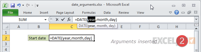
But sometimes you might want to have Excel add placeholders for all the function arguments at once.
If so, you’ll be glad to know that there’s a shortcut for that.

When that happens, remember thatyou can move the hint window out of your way.
Then you could continue entering or editing your formula.
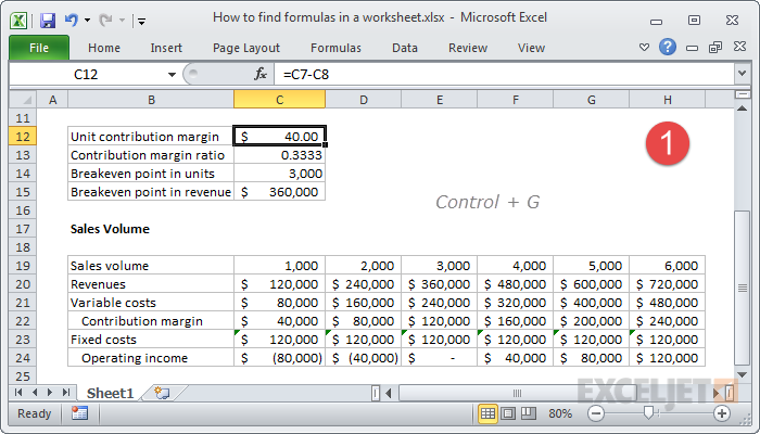
But sometimes you might want to see all of the formulas on a worksheet at one time.

With this shortcut, you might rapidly toggle the display of all formulas on a worksheet or off.
This is a nice way to see all formulas at once, and to check formulas for consistency.
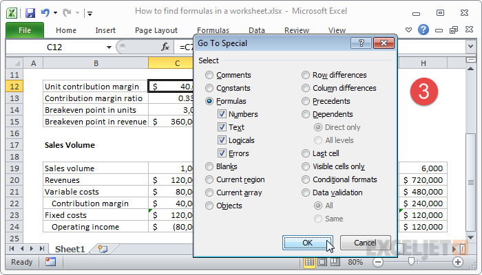
One of the options is cells that contain formulas.

When you click OK, all cells that contain formulas will be selected.
The solution is to first convert formulas to values, then delete the extra columns.
The simplest way to do that is to use Paste Special.

First, go for the formulas you want to convert and Copy to the clipboard.
This will replace all formulas you selected with the values they had calculated.
Next, select all of the dates you want to change.
Then, use Paste Special > Operations > Add.
To increase a set of prices by 10%, use the same approach.
Enter 1.10 into a cell, and copy it to the clipboard.
Once you get the hang of this tip, you’ll find lots of clever uses for it.
Note: this only works with values.
Don’t try it with formulas!

For example, let’s say you have a simple worksheet that shows hours worked for a small team.
For each person, you want to multiply their hours worked times a single hourly rate.
Naming ranges is easy.

As a bonus, you could also easily navigate to the named range whenever you like.
Just go for the name from the drop-down that appears next to the name box.
Excel won’t make any changes to your existing formulas or offer to apply the new range names automatically.

However, there is a way to apply range names to existing formulas.
Just snag the formulas you want to apply names to, then use the Apply Names feature.
Unfortunately, Excel won’t let you enter a formula that’s broken.

However, there’s an easy workaround: just temporarily convert the formula to text.
In both cases, Excel will stop trying to evaluate the formula and will let you enter it as-is.
Later, you’ve got the option to come back to the formula and resume work.
Be aware of the functions that Excel offers
Functions exist to solve specific problems.
For example, the PROPER function has just one purpose: it capitalizes words.
For reference, see ourExcel Function Guideand our list of500 Excel Formula Examples.

Note: People are often confused by the terminology used to talk about functions and formulas.
By this definition, all functions are formulas too, and formulas can contain multiple functions.
Simply put the cursor into a reference and use the shortcut.
Remember that formulas and functions return a value.
Whenever you hear the word “return” with formula, just think “result”.
once you nail a selection, press F9.

You’ll see that part of the formula replaced by the value it returns.
To exit the formula without making changes, just use Esc.
Video:How to check and debug a formula with F9
22.

Evaluate Formula solves a formula one step at a time.
To use Evaluate Formula, select a formula, and tap the button on the ribbon.
One part of the formula will be underlined this is the part currently “under evaluation”.

When you click evaluate, the underlined portion of the formula is replaced with the value it returns.
it’s possible for you to keep clicking evaluate until the formula is fully solved.
Then add in more logic to replace the hard-coded values one step at a time.
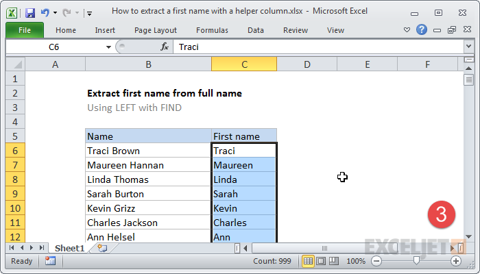
Start with LEFT(full_name, 5) to get the formula working.
Then figure out how to replace the number 5 with a calculated value.
Video:How to build a complex formula step by step
24.

This idea is a little hard to explain sosee this video for a detailed example.
Video:clarify assumptions with concatenation
26.
As you wrangle the parentheses, it is easy to make a mistake in the logic.

This will make the formula read more like a table.
Video:How to make nested IFs easier to read
27.
The trick is to use the tab key.

AutoSum works for both rows and columns.
Excel will guess the range you are trying to sum and insert the SUM function in one step.
AutoSum will even insert multiple SUM functions at the same time.

To sum multiple columns, select a range of empty cells below the columns.
you could actually do this in one step with the keyboard shortcut Control + Enter.
Then, when you’re done, instead of pressing Enter, press Control + Enter.

Excel will add the same formula to all cells in the selection, adjusting references as needed.
You’re done in one step.
it’s possible for you to also use this same technique to edit multiple formulas at the same time.


